Event Study: Texting Bans and Traffic Fatalities
A complete worked example using FARS data
Overview
This worked example walks through a complete event study analysis examining whether state texting-while-driving bans reduced traffic fatalities. We'll use data from the Fatality Analysis Reporting System (FARS), which records all fatal motor vehicle crashes in the United States.
Research Question
Did state laws banning texting while driving reduce traffic fatalities? States adopted these bans at different times between 2007 and 2020, providing staggered variation for a difference-in-differences/event study design.
What We'll Do
- Download FARS data programmatically from NHTSA
- Aggregate to state-year fatality counts
- Merge with texting ban effective dates
- Run event study regression with two-way fixed effects
- Visualize the event study coefficients
Project Setup
Create a directory structure for this project:
* Create project directories
mkdir "texting-bans"
cd "texting-bans"
mkdir "data/raw"
mkdir "data/clean"
mkdir "output"
# Create project directories
dir.create("texting-bans/data/raw", recursive = TRUE)
dir.create("texting-bans/data/clean", recursive = TRUE)
dir.create("texting-bans/output", recursive = TRUE)
setwd("texting-bans")import os
from pathlib import Path
# Create project directories
for d in ["data/raw", "data/clean", "output"]:
Path(f"texting-bans/{d}").mkdir(parents=True, exist_ok=True)
os.chdir("texting-bans")Download Data
NHTSA provides FARS data as downloadable CSV files for each year. We'll download data from 2007-2022 to have adequate pre- and post-periods for most states.
Data Source
The Fatality Analysis Reporting System (FARS) is a nationwide census of fatal motor vehicle crashes. Each row in the accident.csv file represents one fatal crash, with variables for state, date, number of fatalities, and crash characteristics.
Download FARS Files
Download the accident files for each year. These are large files (~20-30MB each), so this may take a few minutes.
* Download FARS data for each year
* Note: Stata doesn't have built-in URL downloading, so we use shell commands

local years 2007 2008 2009 2010 2011 2012 2013 2014 2015 2016 2017 2018 2019 2020 2021 2022

foreach year of local years {
    * Download ZIP file
    shell curl -s -L -o "data/raw/FARS`year'.zip" ///
        "https://static.nhtsa.gov/nhtsa/downloads/FARS/`year'/National/FARS`year'NationalCSV.zip"

    * Extract just the accident.csv file
    shell unzip -j -o "data/raw/FARS`year'.zip" "*/accident.csv" ///
        -d "data/raw/" && mv "data/raw/accident.csv" "data/raw/accident_`year'.csv"

    display "Downloaded `year'"
}
# Download FARS data for each year
pacman::p_load(tidyverse)
years <- 2007:2022
for (year in years) {
url <- paste0("https://static.nhtsa.gov/nhtsa/downloads/FARS/",
year, "/National/FARS", year, "NationalCSV.zip")
zip_file <- paste0("data/raw/FARS", year, ".zip")
# Download ZIP file
download.file(url, zip_file, mode = "wb", quiet = TRUE)
# Extract accident.csv
unzip(zip_file, exdir = "data/raw/temp")
# Find and rename the accident file
accident_file <- list.files("data/raw/temp", pattern = "accident.csv",
recursive = TRUE, full.names = TRUE)
file.rename(accident_file, paste0("data/raw/accident_", year, ".csv"))
# Clean up
unlink("data/raw/temp", recursive = TRUE)
message("Downloaded ", year)
}import requests
import zipfile
import io
import glob
years = range(2007, 2023)
for year in years:
url = (f"https://static.nhtsa.gov/nhtsa/downloads/FARS/"
f"{year}/National/FARS{year}NationalCSV.zip")
# Download ZIP file
r = requests.get(url)
r.raise_for_status()
# Extract accident.csv from the ZIP
with zipfile.ZipFile(io.BytesIO(r.content)) as z:
# Find the accident file (path varies by year)
accident_name = [f for f in z.namelist()
if f.lower().endswith("accident.csv")][0]
# Extract and rename
with z.open(accident_name) as src, \
open(f"data/raw/accident_{year}.csv", "wb") as dst:
dst.write(src.read())
print(f"Downloaded {year}")Load and Combine Years
Now load and append all years into a single dataset:
* Load and append all years
clear
tempfile combined
save `combined', emptyok

forvalues year = 2007/2022 {
    import delimited "data/raw/accident_`year'.csv", clear

    * Keep only variables we need (FARS uses uppercase column names)
    keep STATE STATENAME YEAR MONTH FATALS
    rename *, lower

    append using `combined'
    save `combined', replace
}

use `combined', clear
save "data/clean/fars_all_years.dta", replace

* Check the data
tab year
summarize fatals
# Load and combine all years
pacman::p_load(tidyverse)
fars_list <- list()
for (year in 2007:2022) {
fars_list[[as.character(year)]] <- read_csv(
paste0("data/raw/accident_", year, ".csv"),
show_col_types = FALSE
) %>%
select(STATE, STATENAME, YEAR, MONTH, FATALS) %>%
rename_all(tolower)
}
fars_data <- bind_rows(fars_list)
# Save combined data
write_csv(fars_data, "data/clean/fars_all_years.csv")
# Check the data
fars_data %>% count(year)
fars_data %>% summarize(mean_fatals = mean(fatals),
total_fatals = sum(fatals))import pandas as pd
# Load and combine all years
frames = []
for year in range(2007, 2023):
df = pd.read_csv(f"data/raw/accident_{year}.csv",
usecols=["STATE", "STATENAME", "YEAR", "MONTH", "FATALS"])
frames.append(df)
fars_data = pd.concat(frames, ignore_index=True)
fars_data.columns = fars_data.columns.str.lower()
# Save combined data
fars_data.to_csv("data/clean/fars_all_years.csv", index=False)
# Check the data
print(fars_data.groupby("year").size())
print(fars_data["fatals"].describe())Clean and Aggregate
The raw FARS data has one row per crash. For our event study, we need state-year totals. We'll also need to calculate fatality rates (per capita or per VMT) to account for population differences across states.
Aggregate to State-Year
use "data/clean/fars_all_years.dta", clear

* Collapse to state-year totals
collapse (sum) fatalities = fatals (count) n_crashes = fatals, by(state statename year)

* Label variables
label variable fatalities "Total fatalities"
label variable n_crashes "Number of fatal crashes"

* Check for missing state-years (there shouldn't be any)
egen state_id = group(state)
tsset state_id year
tsfill, full

* Summary statistics
summarize fatalities n_crashes

save "data/clean/state_year_fatalities.dta", replace
# Aggregate to state-year totals
state_year <- fars_data |>
group_by(state, statename, year) |>
summarize(
fatalities = sum(fatals),
n_crashes = n(),
.groups = "drop"
)
# Check for missing state-years
state_year |>
complete(state, year = 2007:2022) |>
filter(is.na(fatalities))
# Summary statistics
summary(state_year$fatalities)
write_csv(state_year, "data/clean/state_year_fatalities.csv")# Aggregate to state-year totals
state_year = (fars_data
.groupby(["state", "statename", "year"])
.agg(fatalities=("fatals", "sum"),
n_crashes=("fatals", "count"))
.reset_index())
# Check for missing state-years
import itertools
all_combos = pd.DataFrame(
itertools.product(state_year["state"].unique(), range(2007, 2023)),
columns=["state", "year"]
)
missing = all_combos.merge(state_year, on=["state", "year"], how="left")
print("Missing state-years:", missing["fatalities"].isna().sum())
# Summary statistics
print(state_year["fatalities"].describe())
state_year.to_csv("data/clean/state_year_fatalities.csv", index=False)Add Population Data (Optional)
For a more rigorous analysis, you'd want to calculate fatality rates per 100,000 population. You can get state population data from the Census Bureau's API or from FRED.
Why Rates Matter (Even with State Fixed Effects)
State fixed effects already absorb time-invariant differences in population levels (Texas is always bigger than Vermont). The concern is differential population growth over the study period. If fast-growing states adopted texting bans at different times than slow-growing states, raw fatality counts could confound population trends with policy effects. Per-capita rates address this by removing variation due to changing population size.
Merge Policy Dates
Now we merge in the texting ban effective dates. The key variable is the year each state's ban went into effect.
Policy Data
First, download the policy dates file (compiled from GHSA and IIHS sources):
* Load policy dates
* Download from: theodorecaputi.com/teaching/14.33/tutorial/worked-examples/texting_ban_dates.csv
import delimited "data/raw/texting_ban_dates.csv", clear

* Handle missing values for states without a ban (Montana, Missouri)
* If CSV has "NA", import delimited reads it as a string; convert to numeric
destring texting_ban_year, replace force

save "data/clean/texting_ban_dates.dta", replace

* Preview the data
list state state_name texting_ban_year primary_enforcement in 1/10
# Load policy dates
# Download from: theodorecaputi.com/teaching/14.33/tutorial/worked-examples/texting_ban_dates.csv
policy <- read_csv("data/raw/texting_ban_dates.csv",
na = c("", "NA", "."),
show_col_types = FALSE)
# Preview
head(policy, 10)# Load policy dates
# Download from: theodorecaputi.com/teaching/14.33/tutorial/worked-examples/texting_ban_dates.csv
policy = pd.read_csv("data/raw/texting_ban_dates.csv",
na_values=["", "NA", "."])
# Preview
print(policy.head(10))Policy Data Format
The texting_ban_dates.csv file contains the following columns:
- state: Numeric FIPS code (1-56) matching the FARS
statecolumn - state_name: Full state name (e.g., "Alabama", "Montana")
- texting_ban_year: Year the texting ban took effect (NA for states without a ban)
- primary_enforcement: 1 if the ban has primary enforcement (police can stop drivers solely for texting), 0 if secondary enforcement only
Montana and Missouri (which only banned texting for drivers under 21, not a statewide comprehensive ban) have texting_ban_year set to NA. The state column uses numeric FIPS codes that match the FARS data, making the merge straightforward.
Merge and Create Treatment Variables
* Merge fatality data with policy dates
use "data/clean/state_year_fatalities.dta", clear
merge m:1 state using "data/clean/texting_ban_dates.dta"

* Check merge
tab _merge
drop _merge

* Create treatment indicator
gen treated = (year >= texting_ban_year) & !missing(texting_ban_year)

* Create event time variable (years since treatment)
gen event_time = year - texting_ban_year

* For never-treated states (Montana, Missouri), set event_time to a placeholder
replace event_time = -999 if missing(texting_ban_year)

* Tabulate treatment timing
tab texting_ban_year, missing
tab event_time if event_time != -999

save "data/clean/analysis_data.dta", replace
# Merge fatality data with policy dates
analysis_data <- state_year %>%
merge(policy, by = "state", all.x = TRUE) %>%
mutate(
# Ever-treated indicator (1 if state ever adopts, 0 if never)
ever_treated = !is.na(texting_ban_year),
# Currently treated indicator
treated = ever_treated & year >= texting_ban_year,
# Event time (years since treatment)
# IMPORTANT: Never-treated states don't have a meaningful "event time"
# Set them to -1000 (a value outside the range of real event times)
# Then exclude with ref = c(-1, -1000) in fixest
event_time = if_else(
is.na(texting_ban_year),
-1000, # Never-treated: code as -1000
year - texting_ban_year # Treated: actual event time
)
)
# Check treatment timing
analysis_data %>% count(texting_ban_year)
analysis_data %>% filter(event_time != -1000) %>% count(event_time)
write_csv(analysis_data, "data/clean/analysis_data.csv")import numpy as np
# Merge fatality data with policy dates
analysis_data = state_year.merge(policy, on="state", how="left")
# Ever-treated indicator
analysis_data["ever_treated"] = analysis_data["texting_ban_year"].notna()
# Currently treated indicator
analysis_data["treated"] = (analysis_data["ever_treated"] &
(analysis_data["year"] >= analysis_data["texting_ban_year"]))
# Event time (years since treatment)
# Never-treated states get -1000 (outside real event-time range)
analysis_data["event_time"] = np.where(
analysis_data["texting_ban_year"].isna(),
-1000,
analysis_data["year"] - analysis_data["texting_ban_year"]
).astype(int)
# Check treatment timing
print(analysis_data.groupby("texting_ban_year", dropna=False).size())
print(analysis_data.query("event_time != -1000")
.groupby("event_time").size())
analysis_data.to_csv("data/clean/analysis_data.csv", index=False)Event Time
event_time = year - texting_ban_year measures years relative to treatment. Negative values are pre-treatment, zero is the treatment year, and positive values are post-treatment. This is the key variable for our event study.
Merge Economic Controls
State and year fixed effects control for time-invariant state characteristics and common year shocks, but they don't control for things that vary both across states and over time. If economic conditions differ across states and correlate with when states adopt texting bans, we could have a problem. We'll add state-level unemployment and per capita income from FRED.
* Download state unemployment and income from FRED
* Each state has a series like "ALUR" (Alabama), "AKUR" (Alaska), etc.
* We download each, extract the annual average, and merge.

* State abbreviations and their FIPS codes (FARS uses FIPS, not sequential IDs)
local st_abbr AL AK AZ AR CA CO CT DE FL GA HI ID IL IN IA KS KY LA ME MD MA MI MN MS MO MT NE NV NH NJ NM NY NC ND OH OK OR PA RI SC SD TN TX UT VT VA WA WV WI WY
local st_fips  1  2  4  5  6  8  9 10 12 13 15 16 17 18 19 20 21 22 23 24 25 26 27 28 29 30 31 32 33 34 35 36 37 38 39 40 41 42 44 45 46 47 48 49 50 51 53 54 55 56

* --- Download unemployment (series: [ST]UR) ---
tempfile unemp_all
clear
gen state = .
gen year = .
gen unemployment = .
save `unemp_all', replace

local n : word count `st_abbr'
forvalues j = 1/`n' {
    local st : word `j' of `st_abbr'
    local fips : word `j' of `st_fips'
    capture {
        local url "https://fred.stlouisfed.org/graph/fredgraph.csv?id=`st'UR"
        copy "`url'" "data/raw/fred_temp.csv", replace
        import delimited "data/raw/fred_temp.csv", clear varnames(1)
        gen year = real(substr(date, 1, 4))
        rename *ur unemployment_val
        keep if year >= 2007 & year <= 2022
        collapse (mean) unemployment = unemployment_val, by(year)
        gen state = `fips'
        append using `unemp_all'
        save `unemp_all', replace
    }
}

* --- Download per capita income (series: [ST]PCPI) ---
tempfile income_all
clear
gen state = .
gen year = .
gen income = .
save `income_all', replace

forvalues j = 1/`n' {
    local st : word `j' of `st_abbr'
    local fips : word `j' of `st_fips'
    capture {
        local url "https://fred.stlouisfed.org/graph/fredgraph.csv?id=`st'PCPI"
        copy "`url'" "data/raw/fred_temp.csv", replace
        import delimited "data/raw/fred_temp.csv", clear varnames(1)
        gen year = real(substr(date, 1, 4))
        rename *pcpi income_val
        keep if year >= 2007 & year <= 2022
        collapse (mean) income = income_val, by(year)
        gen state = `fips'
        append using `income_all'
        save `income_all', replace
    }
}

* Merge to analysis data
use "data/clean/analysis_data.dta", clear
merge 1:1 state year using `unemp_all', nogen keep(master match)
merge 1:1 state year using `income_all', nogen keep(master match)

save "data/clean/analysis_data.dta", replace
# Download state unemployment and income from FRED
# Each state has a FRED series: e.g., "ALUR" for Alabama unemployment
pacman::p_load(tidyverse)
# Load state FIPS mapping (maps numeric FIPS codes to state abbreviations)
state_fips_map <- read_csv("state_fips_map.csv", show_col_types = FALSE)
# Download unemployment (series: [ST]UR)
unemp_frames <- list()
for (i in seq_len(nrow(state_fips_map))) {
st <- state_fips_map$state_abbr[i]
url <- paste0("https://fred.stlouisfed.org/graph/fredgraph.csv?id=", st, "UR")
tryCatch({
df <- read_csv(url, show_col_types = FALSE)
names(df) <- c("date", "unemployment")
df <- df %>%
mutate(year = as.integer(substr(date, 1, 4))) %>%
filter(year >= 2007, year <= 2022) %>%
group_by(year) %>%
summarise(unemployment = mean(unemployment, na.rm = TRUE)) %>%
mutate(state = state_fips_map$state[i])
unemp_frames[[length(unemp_frames) + 1]] <- df
}, error = function(e) NULL)
}
all_unemp <- bind_rows(unemp_frames)
# Download per capita income (series: [ST]PCPI)
income_frames <- list()
for (i in seq_len(nrow(state_fips_map))) {
st <- state_fips_map$state_abbr[i]
url <- paste0("https://fred.stlouisfed.org/graph/fredgraph.csv?id=", st, "PCPI")
tryCatch({
df <- read_csv(url, show_col_types = FALSE)
names(df) <- c("date", "income")
df <- df %>%
mutate(year = as.integer(substr(date, 1, 4))) %>%
filter(year >= 2007, year <= 2022) %>%
group_by(year) %>%
summarise(income = mean(income, na.rm = TRUE)) %>%
mutate(state = state_fips_map$state[i])
income_frames[[length(income_frames) + 1]] <- df
}, error = function(e) NULL)
}
all_income <- bind_rows(income_frames)
# Merge controls to analysis data
analysis_data <- analysis_data %>%
merge(all_unemp, by = c("state", "year"), all.x = TRUE) %>%
merge(all_income, by = c("state", "year"), all.x = TRUE)
write_csv(analysis_data, "data/clean/analysis_data.csv")# Download state unemployment and income from FRED
# Each state has a FRED series: e.g., "ALUR" for Alabama unemployment
state_codes = [
"AL", "AK", "AZ", "AR", "CA", "CO", "CT", "DE", "FL", "GA",
"HI", "ID", "IL", "IN", "IA", "KS", "KY", "LA", "ME", "MD",
"MA", "MI", "MN", "MS", "MO", "MT", "NE", "NV", "NH", "NJ",
"NM", "NY", "NC", "ND", "OH", "OK", "OR", "PA", "RI", "SC",
"SD", "TN", "TX", "UT", "VT", "VA", "WA", "WV", "WI", "WY"
]
state_fips = [
1, 2, 4, 5, 6, 8, 9, 10, 12, 13,
15, 16, 17, 18, 19, 20, 21, 22, 23, 24,
25, 26, 27, 28, 29, 30, 31, 32, 33, 34,
35, 36, 37, 38, 39, 40, 41, 42, 44, 45,
46, 47, 48, 49, 50, 51, 53, 54, 55, 56
]
# Download unemployment (series: [ST]UR)
unemp_frames = []
for st, fips in zip(state_codes, state_fips):
try:
url = f"https://fred.stlouisfed.org/graph/fredgraph.csv?id={st}UR"
df = pd.read_csv(url, parse_dates=["DATE"])
df.columns = ["date", "unemployment"]
df["year"] = df["date"].dt.year
df = (df.query("2007 <= year <= 2022")
.groupby("year")["unemployment"].mean()
.reset_index())
df["state"] = fips
unemp_frames.append(df)
except Exception:
pass
all_unemp = pd.concat(unemp_frames, ignore_index=True)
# Download per capita income (series: [ST]PCPI)
income_frames = []
for st, fips in zip(state_codes, state_fips):
try:
url = f"https://fred.stlouisfed.org/graph/fredgraph.csv?id={st}PCPI"
df = pd.read_csv(url, parse_dates=["DATE"])
df.columns = ["date", "income"]
df["year"] = df["date"].dt.year
df = (df.query("2007 <= year <= 2022")
.groupby("year")["income"].mean()
.reset_index())
df["state"] = fips
income_frames.append(df)
except Exception:
pass
all_income = pd.concat(income_frames, ignore_index=True)
# Merge to analysis data
analysis_data = (analysis_data
.merge(all_unemp, on=["state", "year"], how="left")
.merge(all_income, on=["state", "year"], how="left"))
analysis_data.to_csv("data/clean/analysis_data.csv", index=False)Event Study Regression
An event study estimates separate effects for each time period relative to treatment. This lets us (1) test for pre-trends and (2) trace out the dynamic treatment effect.
The Model
We estimate:
Yst = αs + γt + ∑k≠-1 βk × 1[Kst = k] + Xstδ + εst
Where:
- αs = state fixed effects
- γt = year fixed effects
- Kst = event time (years since treatment)
- βk = effect at event time k, relative to k = -1
- Xst = time-varying controls (unemployment, income)
Create Event Time Dummies
use "data/clean/analysis_data.dta", clear

* Bin endpoints (combine -6 and earlier, +6 and later)
gen event_time_binned = event_time
replace event_time_binned = -6 if event_time <= -6 & event_time != -999
replace event_time_binned = 6 if event_time >= 6 & event_time != -999

* Create dummies for each event time (excluding -1 as reference)
* For never-treated states, all dummies are 0
forvalues k = -6/6 {
    if `k' != -1 {
        local klab = cond(`k' < 0, "m" + string(abs(`k')), "p" + string(`k'))
        gen et_`klab' = (event_time_binned == `k') & (event_time != -999)
    }
}

* Verify: never-treated states should have all zeros
summarize et_* if missing(texting_ban_year)
# In fixest, we use the bin argument inside i() to bin endpoints
# instead of manually creating a binned variable with case_when.
# This is cleaner and less error-prone.
#
# Why -1000 for never-treated?
# Never-treated states don't have a treatment year, so "years since treatment"
# is undefined. We can't just drop them (we need them as controls).
# By coding them as -1000 and including -1000 in ref, fixest:
# 1. Keeps them in the regression (they contribute to fixed effects)
# 2. Doesn't create a dummy for them (no event_time = -1000 coefficient)# Bin endpoints (but keep never-treated at -1000)
analysis_data["event_time_binned"] = np.where(
analysis_data["event_time"] == -1000, -1000,
np.clip(analysis_data["event_time"], -6, 6)
)
# Create dummies for each event time (excluding -1 as reference)
# Never-treated states (event_time == -1000) get 0 for all dummies
for k in range(-6, 7):
if k == -1:
continue # skip reference period
label = f"et_m{abs(k)}" if k < 0 else f"et_p{k}"
analysis_data[label] = ((analysis_data["event_time_binned"] == k) &
(analysis_data["event_time"] != -1000)).astype(int)
# Verify: never-treated states should have all zeros
et_cols = [c for c in analysis_data.columns if c.startswith("et_")]
print(analysis_data.loc[analysis_data["event_time"] == -1000, et_cols].sum())Run the Event Study
* Install reghdfe if needed
* ssc install reghdfe
* ssc install ftools

* Log transform outcome (fatalities are count data)
gen ln_fatalities = ln(fatalities)

* Event study with two-way fixed effects
reghdfe ln_fatalities et_m6 et_m5 et_m4 et_m3 et_m2 ///
    et_p0 et_p1 et_p2 et_p3 et_p4 et_p5 et_p6 ///
    unemployment income, ///
    absorb(state year) cluster(state)

* Store estimates for plotting
estimates store event_study

* Display results
esttab event_study, se keep(et_*) ///
    title("Event Study: Effect of Texting Bans on Log Fatalities")

* Alternative: xtevent simplifies event studies
* ssc install xtevent
* xtevent ln_fatalities unemployment income, ///
*     policyvar(treated) panelvar(state) timevar(year) ///
*     window(6) cluster(state)
* xteventplot, title("Event Study: Texting Bans (xtevent)")
# Install fixest if needed
# install.packages("fixest")
pacman::p_load(fixest, ggfixest)
# Log transform outcome
analysis_data <- analysis_data %>%
mutate(ln_fatalities = log(fatalities))
# Event study with two-way fixed effects
# i(event_time, ...) creates event-time dummies
# bin = .("-6+" = ~x <= -6, "6+" = ~x >= 6) bins the endpoints
# ref = c(-1, -1000) excludes t=-1 (reference) AND t=-1000 (never-treated)
#
# See: https://lrberge.github.io/fixest/articles/fixest_walkthrough.html
event_study <- feols(
ln_fatalities ~ i(event_time, ever_treated, ref = c(-1, -1000),
bin = .("-6+" = ~x <= -6, "6+" = ~x >= 6)) +
unemployment + income | state + year,
data = analysis_data,
cluster = ~state
)
# Display results
summary(event_study)# pip install linearmodels
from linearmodels.panel import PanelOLS
# Log transform outcome
analysis_data["ln_fatalities"] = np.log(analysis_data["fatalities"])
# Set panel index
panel = analysis_data.set_index(["state", "year"])
# Event time dummy columns (already created above)
et_cols = [c for c in analysis_data.columns if c.startswith("et_")]
# Event study with two-way fixed effects
formula = "ln_fatalities ~ " + " + ".join(et_cols) + " + unemployment + income + EntityEffects + TimeEffects"
model = PanelOLS.from_formula(formula, data=panel)
event_study = model.fit(cov_type="clustered", cluster_entity=True)
print(event_study.summary)Standard Errors
We cluster standard errors at the state level because (1) treatment varies at the state level, and (2) fatalities within a state are likely correlated over time. This is essential for correct inference in DiD designs.
Results
The event study coefficients (relative to t = −1) with 95% confidence intervals:
| Event Time | Coefficient | Std. Error | 95% CI Lower | 95% CI Upper |
|---|---|---|---|---|
| −6 | −0.0510 | 0.0469 | −0.1431 | 0.0411 |
| −5 | −0.0141 | 0.0274 | −0.0680 | 0.0398 |
| −4 | −0.0187 | 0.0191 | −0.0562 | 0.0187 |
| −3 | −0.0055 | 0.0191 | −0.0430 | 0.0319 |
| −2 | 0.0085 | 0.0167 | −0.0243 | 0.0414 |
| −1 | 0.0000 | — | — | — |
| 0 | 0.0221 | 0.0191 | −0.0153 | 0.0595 |
| 1 | 0.0126 | 0.0207 | −0.0281 | 0.0533 |
| 2 | 0.0115 | 0.0262 | −0.0400 | 0.0630 |
| 3 | 0.0135 | 0.0279 | −0.0413 | 0.0683 |
| 4 | 0.0115 | 0.0343 | −0.0558 | 0.0788 |
| 5 | 0.0068 | 0.0330 | −0.0580 | 0.0717 |
| 6 | 0.0063 | 0.0372 | −0.0667 | 0.0793 |
Reference period: t = −1. Standard errors clustered at the state level.
Visualization
The classic event study plot shows coefficients and confidence intervals for each event time, with the reference period (t = -1) normalized to zero.
* Install coefplot if needed
* ssc install coefplot

* Create event study plot
coefplot event_study, ///
    keep(et_*) ///
    vertical ///
    yline(0, lcolor(red) lpattern(dash)) ///
    xline(5.5, lcolor(gray) lpattern(dash)) ///
    xlabel(1 "-6" 2 "-5" 3 "-4" 4 "-3" 5 "-2" ///
           6 "0" 7 "1" 8 "2" 9 "3" 10 "4" 11 "5" 12 "6") ///
    xtitle("Years Relative to Texting Ban") ///
    ytitle("Effect on Log Fatalities") ///
    title("Event Study: Texting Bans and Traffic Fatalities") ///
    note("Notes: Coefficients relative to t=-1. 95% CIs shown." ///
         "Clustered SEs at state level.") ///
    ciopts(recast(rcap)) ///
    msymbol(D) mcolor(navy) ///
    graphregion(color(white)) bgcolor(white)

graph export "output/event_study.png", replace width(1200)
# Quick event study plot with ggiplot (one line!)
pacman::p_load(ggfixest)
p <- ggiplot(event_study,
xlab = "Years Relative to Texting Ban",
ylab = "Effect on Log Fatalities",
main = "Event Study: Texting Bans and Traffic Fatalities")
ggsave("output/event_study_quick.png", p, width = 10, height = 6, dpi = 300)
# For a more customized publication-quality plot:
pacman::p_load(broom, ggplot2)
# Extract coefficients
coef_df <- tidy(event_study, conf.int = TRUE) %>%
filter(str_detect(term, "event_time")) %>%
mutate(
event_time = as.numeric(str_extract(term, "-?\\d+"))
) %>%
# Add the reference period (t = -1)
bind_rows(tibble(event_time = -1, estimate = 0,
conf.low = 0, conf.high = 0))
# Create plot
p <- ggplot(coef_df, aes(x = event_time, y = estimate)) +
geom_hline(yintercept = 0, linetype = "dashed", color = "red") +
geom_vline(xintercept = -0.5, linetype = "dashed", color = "gray") +
geom_pointrange(aes(ymin = conf.low, ymax = conf.high)) +
labs(
x = "Years Relative to Texting Ban",
y = "Effect on Log Fatalities",
title = "Event Study: Texting Bans and Traffic Fatalities",
caption = "Notes: Coefficients relative to t=-1. 95% CIs shown.\nClustered SEs at state level."
) +
theme_minimal() +
theme(
panel.grid.minor = element_blank(),
plot.title = element_text(hjust = 0.5)
)
ggsave("output/event_study.png", p, width = 10, height = 6, dpi = 300)import matplotlib.pyplot as plt
# Extract coefficients and confidence intervals
et_order = ["et_m6", "et_m5", "et_m4", "et_m3", "et_m2",
"et_p0", "et_p1", "et_p2", "et_p3", "et_p4", "et_p5", "et_p6"]
event_times = [-6, -5, -4, -3, -2, 0, 1, 2, 3, 4, 5, 6]
coefs = [event_study.params[c] for c in et_order]
ci_lower = [event_study.conf_int().loc[c, "lower"] for c in et_order]
ci_upper = [event_study.conf_int().loc[c, "upper"] for c in et_order]
# Add reference period (t = -1)
event_times.insert(5, -1)
coefs.insert(5, 0)
ci_lower.insert(5, 0)
ci_upper.insert(5, 0)
# Plot
fig, ax = plt.subplots(figsize=(10, 6))
ax.axhline(0, color="red", linestyle="--", linewidth=0.8)
ax.axvline(-0.5, color="gray", linestyle="--", linewidth=0.8)
ax.errorbar(event_times, coefs,
yerr=[
[c - lo for c, lo in zip(coefs, ci_lower)],
[hi - c for c, hi in zip(coefs, ci_upper)]
],
fmt="D", color="navy", capsize=4, markersize=5)
ax.set_xlabel("Years Relative to Texting Ban")
ax.set_ylabel("Effect on Log Fatalities")
ax.set_title("Event Study: Texting Bans and Traffic Fatalities")
ax.annotate("Coefficients relative to t=-1. 95% CIs shown.\n"
"Clustered SEs at state level.",
xy=(0.5, -0.12), xycoords="axes fraction",
ha="center", fontsize=9, color="gray")
plt.tight_layout()
plt.savefig("output/event_study.png", dpi=300)
plt.show()Output
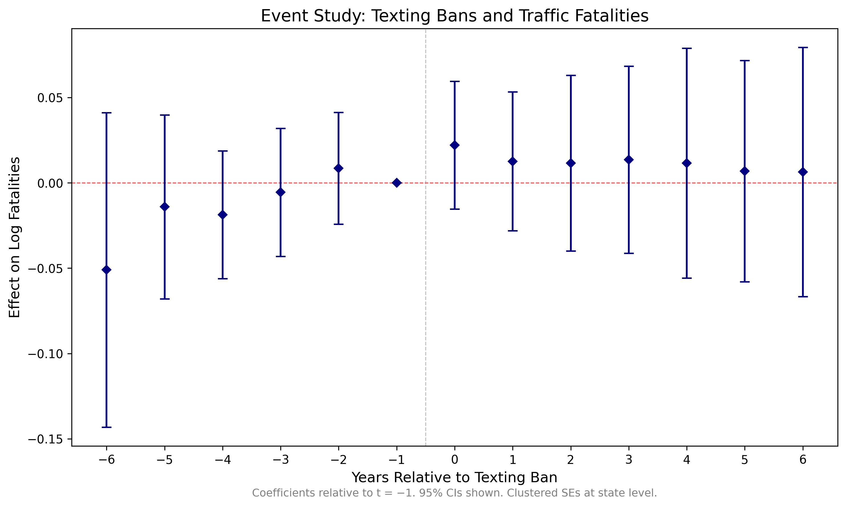
Event study coefficients with 95% confidence intervals. Reference period: t = −1. Clustered standard errors at the state level.
Replication Package
Download a complete replication package that downloads the data, runs the analysis, and produces the event study plot above. Each package includes a master script that runs all steps sequentially.
What's Included
Each package contains the analysis code and texting_ban_dates.csv (in build/input/, 52 rows). FARS data (~400 MB) and FRED economic data are downloaded automatically when you run the master script. The first run takes 15-20 minutes (mostly FARS downloads); subsequent runs use cached data and finish in under a minute.
Interpretation
Reading the Event Study Plot
The event study plot tells us several things:
Pre-Trends
Look at coefficients for t < 0. If they're close to zero and not trending, the parallel trends assumption is more credible. Significant pre-trends suggest treated and control states were already diverging before the law.
Treatment Effect
Look at t = 0 and beyond. Negative coefficients mean the texting ban reduced fatalities. The magnitude tells you the percent change (since our outcome is in logs).
Dynamics
Does the effect appear immediately at t = 0? Does it grow over time? Fade out? These dynamics can be informative about the mechanism.
Null Results Are Results
If you find no effect of texting bans on fatalities, that's a finding. It could mean bans are ineffective, or that enforcement is weak, or that texting wasn't a major cause of fatal crashes. Don't bury null results.
Caveats and Extensions
- Enforcement: Primary vs. secondary enforcement matters. You could interact treatment with enforcement type.
- Spillovers: Drivers cross state lines. Border counties might be affected by neighboring state laws.
- Other policies: Handheld bans, distracted driving laws, and other traffic safety policies may confound results.
Recent research has found that DD estimates can be biased when there is both (A) staggered treatment timing and (B) heterogeneous treatment effects. You don't need to know anything about this for 14.33. If you're interested, ask your TA!
Found something unclear or have a suggestion? Email [email protected].