Complete Project Walkthrough

From raw data to publication-ready output — start to finish

This walkthrough takes you through an entire empirical project: loading data, cleaning, merging multiple datasets, running a difference-in-differences analysis with event study, and producing publication-quality tables and figures. We also cover instrumental variables and regression discontinuity as standalone analyses.

Project Setup

An empirical project separates raw data from processed data, and build code (data processing) from analysis code (regressions, tables, figures). The download below contains the full project with this structure already in place.

Download the Project

Starter packages contain data and empty code files for you to fill in as you follow along. Complete packages include finished code that runs end-to-end.

	Stata	R	Python
Starter	Download	Download	Download
Complete	Download	Download	Download

Tutorial Slides (PDF)

Running Your Scripts

Once you've downloaded and unzipped the project, open a terminal in the project folder and run the master file. You can also run individual scripts for development.

Stata (command line):

Mac: /Applications/Stata/StataMP.app/Contents/MacOS/stata-mp -b do master.do
Windows: "C:\Program Files\Stata18\StataMP-64.exe" /e do master.do
Linux: stata-mp -b do master.do

The -b (Mac/Linux) or /e (Windows) flag runs Stata in batch mode — output goes to a .log file in the working directory instead of the GUI.

Stata (VS Code): Install the Stata Enhanced extension for syntax highlighting and stataRun to run code directly. After installing stataRun, open VS Code settings and set the path to your Stata executable (e.g. /Applications/Stata/StataMP.app/Contents/MacOS/stata-mp). Then open a .do file and press Ctrl+Shift+A (Cmd+Shift+A on Mac) to run the entire file.

R: Run Rscript master.R from the terminal, or open the project in RStudio and source the master file.

Python: Run python master.py from the terminal, or use VS Code with the Python extension to run scripts interactively.

What's Inside

Unzipping gives you a single project folder (e.g. pkg-stata/) with this structure:

pkg-stata/
├── master.do                  ← Runs everything in order
├── build/
│   ├── code/
│   │   ├── 01_filter_crashes.do
│   │   ├── 02_collapse_crashes.do
│   │   ├── 03_reshape_crashes.do
│   │   ├── 04_append_demographics.do
│   │   ├── 05_collapse_demographics.do
│   │   └── 06_merge_datasets.do
│   ├── input/                 ← Raw data (NEVER modified by code)
│   │   ├── crash_data.csv
│   │   ├── demographic_survey/  ← 21 annual CSVs (1995-2015)
│   │   ├── policy_adoptions.csv
│   │   └── state_names.csv
│   └── output/                ← Processed data (created by build scripts)
└── analysis/
    ├── code/
    │   ├── 01_descriptive_table.do
    │   ├── 02_dd_regression.do
    │   ├── 03_event_study.do
    │   ├── 04_dd_table.do
    │   ├── 05_iv.do
    │   └── 06_rd.do
    └── output/
        ├── tables/
        └── figures/

Key Principles

Raw data is read-only. Files in build/input/ are never modified by your code. If you need to clean or transform data, save the result to build/output/.
Build vs. analysis. Build scripts (build/code/) turn raw data into analysis-ready datasets. Analysis scripts (analysis/code/) take those datasets and produce results. This separation means you can change a regression without re-processing all your data.
Numbered scripts. Prefix scripts with 01_, 02_, etc. so the execution order is obvious. A master.do file at the root runs them all sequentially.
Outputs are reproducible. Everything in build/output/ and analysis/output/ can be regenerated by running master.do. Never hand-edit output files.

The Master File

The master.do sets global paths and runs every script in order. Anyone should be able to replicate your results by changing one path and running this file.

* MASTER DO FILE
clear all
set more off

* >>> CHANGE THIS to your project path <<<
global root "/path/to/pkg-stata"
global build "$root/build"
global analysis "$root/analysis"

cd "$root"

* Build stage
do "$build/code/01_filter_crashes.do"
do "$build/code/02_collapse_crashes.do"
do "$build/code/03_reshape_crashes.do"
do "$build/code/04_append_demographics.do"
do "$build/code/05_collapse_demographics.do"
do "$build/code/06_merge_datasets.do"

* Analysis stage
do "$analysis/code/01_descriptive_table.do"
do "$analysis/code/02_dd_regression.do"
do "$analysis/code/03_event_study.do"
do "$analysis/code/04_dd_table.do"
do "$analysis/code/05_iv.do"
do "$analysis/code/06_rd.do"

# master.R
rm(list = ls())

# Set root directory (CHANGE THIS to your project path)
root <- "."
build <- file.path(root, "build")
analysis <- file.path(root, "analysis")

# Build stage
source(file.path(build, "code", "01_filter_crashes.R"))
source(file.path(build, "code", "02_collapse_crashes.R"))
source(file.path(build, "code", "03_reshape_crashes.R"))
source(file.path(build, "code", "04_append_demographics.R"))
source(file.path(build, "code", "05_collapse_demographics.R"))
source(file.path(build, "code", "06_merge_datasets.R"))

# Analysis stage
source(file.path(analysis, "code", "01_descriptive_table.R"))
source(file.path(analysis, "code", "02_dd_regression.R"))
source(file.path(analysis, "code", "03_event_study.R"))
source(file.path(analysis, "code", "04_dd_table.R"))
source(file.path(analysis, "code", "05_iv.R"))
source(file.path(analysis, "code", "06_rd.R"))

# master.py
import subprocess, sys, os

root = "."
build = os.path.join(root, "build")
analysis = os.path.join(root, "analysis")

scripts = [
    f"{build}/code/01_filter_crashes.py",
    f"{build}/code/02_collapse_crashes.py",
    f"{build}/code/03_reshape_crashes.py",
    f"{build}/code/04_append_demographics.py",
    f"{build}/code/05_collapse_demographics.py",
    f"{build}/code/06_merge_datasets.py",
    f"{analysis}/code/01_descriptive_table.py",
    f"{analysis}/code/02_dd_regression.py",
    f"{analysis}/code/03_event_study.py",
    f"{analysis}/code/04_dd_table.py",
    f"{analysis}/code/05_iv.py",
    f"{analysis}/code/06_rd.py",
]

for script in scripts:
    print(f"Running {script}...")
    subprocess.run([sys.executable, script], check=True)

Every raw dataset is a little different, and you'll need to figure out what steps are required to get each one into the format your analysis needs. Parts A and B walk through two examples — cleaning crash data and cleaning demographic survey data — that illustrate common operations (filtering, collapsing, reshaping, looping, appending, destringing). The specific steps will depend on the raw data you're actually working with.

Part A: Cleaning the Crash Data

The crash data has one row per crash, but our analysis is at the state-year level. Scripts 01–03 read the raw data, filter it, collapse it to counts, and reshape it so each severity type gets its own column.

Step 1: Read and Filter Crashes

Start by reading the crash-level CSV. This is granular data we'll need to aggregate.

* Read crash-level data (CSV)
import delimited "$build/input/crash_data.csv", clear
describe
summarize
tab severity

pacman::p_load(data.table)

# Read crash-level data (CSV)
crashes <- fread("build/input/crash_data.csv")
str(crashes)
summary(crashes)
table(crashes$severity)

import pandas as pd

# Read crash-level data (CSV)
crashes = pd.read_csv("build/input/crash_data.csv")
print(crashes.info())
print(crashes.describe())
print(crashes['severity'].value_counts())

Script 01_filter_crashes also drops observations we don't need before any aggregation.

* Load crash data
import delimited "$build/input/crash_data.csv", clear

* --- FILTER: Keep only fatal and serious crashes ---
drop if severity == "minor"

save "$build/output/crashes_filtered.dta", replace

pacman::p_load(data.table)

# Load crash data
crashes <- fread("build/input/crash_data.csv")

# Filter: keep only fatal and serious crashes
crashes <- crashes[severity != "minor"]

fwrite(crashes, "build/output/crashes_filtered.csv")

import pandas as pd

# Load crash data
crashes = pd.read_csv("build/input/crash_data.csv")

# Filter: keep only fatal and serious crashes
crashes = crashes[crashes['severity'] != 'minor']

crashes.to_csv("build/output/crashes_filtered.csv", index=False)

Step 2: Collapse to State-Year-Severity

Script 02_collapse_crashes counts crashes by state, year, and severity type.

use "$build/output/crashes_filtered.dta", clear

* --- COLLAPSE: Count crashes by state-year-severity (long format) ---
gen one = 1
collapse (sum) n_crashes = one, by(state_fips year severity)

save "$build/output/crashes_long.dta", replace

pacman::p_load(data.table)

crashes <- fread("build/output/crashes_filtered.csv")

# Collapse to state-year-severity level (long format)
crashes_long <- crashes[, .(n_crashes = .N), by = .(state_fips, year, severity)]

fwrite(crashes_long, "build/output/crashes_long.csv")

import pandas as pd

crashes = pd.read_csv("build/output/crashes_filtered.csv")

# Collapse to state-year-severity level (long format)
crashes_long = (crashes.groupby(['state_fips', 'year', 'severity'])
                .size().reset_index(name='n_crashes'))

crashes_long.to_csv("build/output/crashes_long.csv", index=False)

Step 3: Reshape and Save

Script 03_reshape_crashes pivots the long data wide, renames columns, computes derived variables, and saves the final crash dataset.

use "$build/output/crashes_long.dta", clear

* --- RESHAPE: Wide so each severity type becomes its own column ---
reshape wide n_crashes, i(state_fips year) j(severity) string

* Rename for clarity
rename n_crashesfatal fatal_crashes
rename n_crashesserious serious_crashes

* Compute total and fatal share
gen total_crashes = fatal_crashes + serious_crashes
gen fatal_share = fatal_crashes / total_crashes

* Save intermediate file
save "$build/output/crashes_state_year.dta", replace
describe

pacman::p_load(data.table)

crashes_long <- fread("build/output/crashes_long.csv")

# Reshape from long to wide: one column per severity type
crashes_sy <- dcast(crashes_long, state_fips + year ~ severity,
                    value.var = "n_crashes", fill = 0L)

# Rename and compute totals
setnames(crashes_sy, c("fatal", "serious"), c("fatal_crashes", "serious_crashes"))
crashes_sy[, total_crashes := fatal_crashes + serious_crashes]
crashes_sy[, fatal_share := fatal_crashes / total_crashes]

# Save intermediate file
fwrite(crashes_sy, "build/output/crashes_state_year.csv")
str(crashes_sy)

import pandas as pd

crashes_long = pd.read_csv("build/output/crashes_long.csv")

# Reshape (pivot) from long to wide: one column per severity type
crashes_sy = crashes_long.pivot_table(
    index=['state_fips', 'year'], columns='severity',
    values='n_crashes', fill_value=0
).reset_index()
crashes_sy.columns.name = None
crashes_sy = crashes_sy.rename(columns={'fatal': 'fatal_crashes',
                                         'serious': 'serious_crashes'})

# Compute total and fatal share
crashes_sy['total_crashes'] = crashes_sy['fatal_crashes'] + crashes_sy['serious_crashes']
crashes_sy['fatal_share'] = crashes_sy['fatal_crashes'] / crashes_sy['total_crashes']

# Save intermediate file
crashes_sy.to_csv("build/output/crashes_state_year.csv", index=False)
print(crashes_sy.info())

Why Save Intermediate Files?

Separating your build code (data processing) from analysis code is a key principle of project organization. Save collapsed data so you can modify your analysis without re-running expensive data processing steps every time.

Part B: Cleaning the Demographics Data

The demographic survey data arrives as 21 separate annual CSV files (one per year, 1995–2015). Scripts 04 and 05 stack them into a single dataset, clean the data, and collapse to the state-year level.

Why Loop and Append?

A lot of public-use data is released as separate annual files. You'll need to loop over the files and append them together before you can do anything else. Writing a loop is far better than manually importing 21 files — it's shorter, less error-prone, and generalizes if files are added later.

Step 4: Loop and Append Demographics

Script 04_append_demographics reads each annual CSV, tags it with the year, and appends all 21 files into one dataset.

* Loop through yearly survey CSV files and append
clear
forvalues y = 1995/2015 {
    preserve
    import delimited "$build/input/demographic_survey/demographic_survey_`y'.csv", clear
    gen year = `y'
    tempfile temp`y'
    save `temp`y''
    restore
    append using `temp`y''
}
save "$build/output/demographics_combined.dta", replace

# Loop through yearly survey CSVs and stack them
files <- list.files("build/input/demographic_survey",
                    pattern = "^demographic_survey_\\d{4}\\.csv$",
                    full.names = TRUE)
demo_list <- lapply(files, function(f) {
  dt <- fread(f)
  dt[, year := as.integer(gsub(".*_(\\d{4})\\.csv$", "\\1", f))]
  dt
})
demo_all <- rbindlist(demo_list)
fwrite(demo_all, "build/output/demographics_combined.csv")

import glob
import pandas as pd

# Read and stack all yearly survey CSVs
files = sorted(glob.glob("build/input/demographic_survey/demographic_survey_*.csv"))
frames = []
for f in files:
    df = pd.read_csv(f)
    year = int(f.split("_")[-1].replace(".csv", ""))
    df["year"] = year
    frames.append(df)
demo_all = pd.concat(frames, ignore_index=True)
demo_all.to_csv("build/output/demographics_combined.csv", index=False)

Step 5: Clean and Collapse Demographics

Script 05_collapse_demographics drops DC and pre-2000 years, cleans the income variable (stored as a string with dollar signs and commas), and collapses to the state-year level using survey weights.

Why Destring Income?

Survey data frequently stores numeric values as strings — "$45,000" instead of 45000. You must strip the formatting characters and convert to numeric before doing any math. This is one of the most common data-cleaning tasks in applied work.

use "$build/output/demographics_combined.dta", clear

* Drop DC and pre-2000 years
drop if state_fips == 51
drop if year < 2000

* Clean income: remove $ and commas, convert to numeric
destring income, replace ignore("$,")

* Collapse to state-year level using survey weights
collapse (rawsum) population = weight ///
    (mean) median_income = income pct_urban = urban ///
    [aweight = weight], by(state_fips year)

save "$build/output/demographics_state_year.dta", replace

demo_all <- fread("build/output/demographics_combined.csv")

# Drop DC and pre-2000
demo_all <- demo_all[state_fips != 51 & year >= 2000]

# Clean income: remove $ and commas
demo_all[, income_num := as.numeric(gsub("[\\$,]", "", income))]

# Weighted collapse to state-year level
demographics <- demo_all[, .(
  population    = sum(weight),
  median_income = weighted.mean(income_num, weight),
  pct_urban     = weighted.mean(urban, weight)
), by = .(state_fips, year)]

fwrite(demographics, "build/output/demographics_state_year.csv")

demo_all = pd.read_csv("build/output/demographics_combined.csv")

# Drop DC and pre-2000
demo_all = demo_all[(demo_all["state_fips"] != 51) & (demo_all["year"] >= 2000)]

# Clean income: remove $ and commas
demo_all["income_num"] = (demo_all["income"]
    .str.replace("$", "", regex=False)
    .str.replace(",", "")
    .astype(float))

# Weighted collapse
def weighted_mean(group, col, wt):
    return (group[col] * group[wt]).sum() / group[wt].sum()

demographics = (demo_all.groupby(["state_fips", "year"])
    .apply(lambda g: pd.Series({
        "population": g["weight"].sum(),
        "median_income": weighted_mean(g, "income_num", "weight"),
        "pct_urban": weighted_mean(g, "urban", "weight"),
    }))
    .reset_index())

demographics.to_csv("build/output/demographics_state_year.csv", index=False)

Part C: Merging Multiple Datasets

Now we merge four datasets together: (1) aggregated crashes, (2) state demographics (from Part C), (3) policy adoption dates, and (4) state names. Each merge uses state_fips as the key, with some using year as well.

* Convert CSVs to .dta for merging
import delimited "$build/input/policy_adoptions.csv", clear
save "$build/output/policy_adoptions.dta", replace

import delimited "$build/input/state_names.csv", clear
save "$build/output/state_names.dta", replace

* Load the main dataset and merge everything sequentially
use "$build/output/crashes_state_year.dta", clear

* Merge 1: Demographics — keep only matched rows
merge 1:1 state_fips year using "$build/output/demographics_state_year.dta", ///
    keep(match) nogen

* Merge 2: Policy adoptions — keep master + matched (some states never adopt)
merge m:1 state_fips using "$build/output/policy_adoptions.dta", ///
    keep(master match) nogen

* Merge 3: State names — keep only matched rows
merge m:1 state_fips using "$build/output/state_names.dta", ///
    keep(match) nogen

* Create treatment indicator
gen post_treated = (year >= adoption_year & !missing(adoption_year))
gen log_pop = ln(population)

* Save final analysis dataset
save "$build/output/analysis_panel.dta", replace
describe

pacman::p_load(data.table)

# Load all datasets
crashes_sy <- fread("build/output/crashes_state_year.csv")
demographics <- fread("build/output/demographics_state_year.csv")
policies <- fread("build/input/policy_adoptions.csv")
state_names <- fread("build/input/state_names.csv")

# Merge 1: Crashes + Demographics (on state_fips + year)
panel <- merge(crashes_sy, demographics, by = c("state_fips", "year"), all = FALSE)
cat("After merge 1:", nrow(panel), "rows\n")

# Merge 2: + Policy adoptions (on state_fips only — many:1)
panel <- merge(panel, policies, by = "state_fips", all.x = TRUE)
cat("After merge 2:", nrow(panel), "rows\n")

# Merge 3: + State names (on state_fips only — many:1)
panel <- merge(panel, state_names, by = "state_fips", all.x = TRUE)
cat("After merge 3:", nrow(panel), "rows\n")

# Create treatment indicator
panel[, post_treated := fifelse(
  !is.na(adoption_year) & year >= adoption_year, 1L, 0L
)]
panel[, log_pop := log(population)]

# Save final analysis dataset
fwrite(panel, "build/output/analysis_panel.csv")
str(panel)

import pandas as pd
import numpy as np

# Load all datasets
crashes_sy = pd.read_csv("build/output/crashes_state_year.csv")
demographics = pd.read_csv("build/output/demographics_state_year.csv")
policies = pd.read_csv("build/input/policy_adoptions.csv")
state_names = pd.read_csv("build/input/state_names.csv")

# Merge 1: Crashes + Demographics (on state_fips + year)
panel = crashes_sy.merge(demographics, on=['state_fips', 'year'], how='inner')
print(f"After merge 1: {len(panel)} rows")

# Merge 2: + Policy adoptions (on state_fips only — many:1)
panel = panel.merge(policies, on='state_fips', how='left')
print(f"After merge 2: {len(panel)} rows")

# Merge 3: + State names (on state_fips only — many:1)
panel = panel.merge(state_names, on='state_fips', how='left')
print(f"After merge 3: {len(panel)} rows")

# Create treatment indicator
panel['post_treated'] = (
    (panel['year'] >= panel['adoption_year']) &
    panel['adoption_year'].notna()
).astype(int)
panel['log_pop'] = np.log(panel['population'])

# Save final analysis dataset
panel.to_csv("build/output/analysis_panel.csv", index=False)
print(panel.info())

Understanding Merge Types

Merges can be deceptively complicated. There are three types:

1:1 — Each row in one dataset matches exactly one row in the other. This is the most common merge. Example: merging two state-year datasets on state_fips and year.
m:1 (many-to-one) — Multiple rows in the master dataset match one row in the using dataset. Example: merging individual-level data with state-level variables. Many individuals share the same state, so each state-level row gets matched to multiple individual rows.
1:m (one-to-many) — The reverse: one row in the master matches many rows in the using dataset.

In the code above, Merge 1 is a 1:1 merge (one row per state-year in both datasets). Merges 2 and 3 are m:1 — the panel has many state-year rows per state, but the policy and state-name files have one row per state.

The `keep()` Option in Stata

In Stata, your original dataset is called "master" and the dataset you're merging in is called "using." After a merge, each observation is one of three types:

master — rows from the master that didn't match anything in the using data
match — rows that matched between master and using
using — rows from the using data that didn't match anything in the master

You choose which to keep with the keep() option. Be careful — the wrong choice silently drops observations.

Example: Suppose you have a balanced state-year panel and want to merge in earthquake counts. You collapse the earthquake data to state-year totals, but states with no earthquakes don't appear in that dataset at all.

* BAD: keep(match) drops states with zero earthquakes!
merge 1:1 state year using "earthquakes.dta", keep(match)

* GOOD: keep(master match) preserves all original observations
merge 1:1 state year using "earthquakes.dta", keep(master match) nogen
replace num_earthquakes = 0 if missing(num_earthquakes)

# BAD: inner join drops states with zero earthquakes
panel <- merge(panel, earthquakes, by = c("state", "year"))

# GOOD: left join preserves all original observations
panel <- merge(panel, earthquakes, by = c("state", "year"), all.x = TRUE)
panel[is.na(num_earthquakes), num_earthquakes := 0]

# BAD: inner join drops states with zero earthquakes
panel = panel.merge(earthquakes, on=['state', 'year'])

# GOOD: left join preserves all original observations
panel = panel.merge(earthquakes, on=['state', 'year'], how='left')
panel['num_earthquakes'] = panel['num_earthquakes'].fillna(0)

The Rule of Thumb

Start with a dataset that contains all the observations you want. Use keep(master match) in Stata (or how='left' in R/Python) almost always. Then replace missing values with the appropriate value (often 0, meaning "no events") for any variable you merged in. This ensures your panel stays balanced and you never silently drop observations.

Always Check Your Merges

After every merge, verify: (1) the number of rows is what you expect, (2) there are no unexpected missing values, and (3) the merge type (1:1, m:1, 1:m) matches your data structure. In Stata, the nogen option suppresses the _merge variable. In R/Python, compare row counts before and after.

Part D: Descriptive Statistics Table

Before running regressions, present a descriptive statistics table. A standard format in DD papers has four columns: (1) all observations, (2) treated states in the post-treatment period, (3) treated states before treatment, and (4) never-treated states. This shows how the groups compare and whether there are large pre-treatment differences.

use "$build/output/analysis_panel.dta", clear

* Create group indicator
gen group = 3 if missing(adoption_year)
replace group = 1 if !missing(adoption_year) & year >= adoption_year
replace group = 2 if !missing(adoption_year) & year < adoption_year

label define grp 1 "Treated After" 2 "Treated Before" 3 "Untreated"
label values group grp

* Encode region for factor variable (dtable requires numeric)
encode region, gen(census_region)
label variable census_region "Census Region"

* Label variables
label variable fatal_crashes "Fatal Crashes"
label variable serious_crashes "Serious Crashes"
label variable total_crashes "Total Crashes"
label variable fatal_share "Fatal Share"
label variable population "Population"
label variable median_income "Median Income"
label variable pct_urban "Pct. Urban"

* dtable produces "mean (sd)" format by default
dtable fatal_crashes serious_crashes total_crashes ///
    fatal_share population median_income pct_urban ///
    i.census_region, ///
    by(group) ///
    nformat(%14.2fc mean sd) ///
    sample(, statistics(freq) place(seplabels))

* Rename "Total" column to "All"
collect label levels group .m "All", modify
collect style header group, title(hide)

* Export LaTeX fragment
collect export "$analysis/output/tables/descriptive_table_raw.tex", tableonly replace

* Strip \begin{table} wrapper (dtable adds it; we just need the tabular)
filefilter "$analysis/output/tables/descriptive_table_raw.tex" ///
    "$analysis/output/tables/descriptive_table_s1.tex", ///
    from("\BSbegin{table}[!h]") to("") replace
filefilter "$analysis/output/tables/descriptive_table_s1.tex" ///
    "$analysis/output/tables/descriptive_table_s2.tex", ///
    from("\BScentering") to("") replace
filefilter "$analysis/output/tables/descriptive_table_s2.tex" ///
    "$analysis/output/tables/descriptive_table.tex", ///
    from("\BSend{table}") to("") replace

pacman::p_load(data.table, modelsummary)

panel <- fread("build/output/analysis_panel.csv")

# Create group column
panel[, ever_treated := !is.na(adoption_year)]
panel[, group := fifelse(
  !ever_treated, "Untreated",
  fifelse(post_treated == 1, "Treated x Post", "Treated x Pre")
)]

# Variables for the table
vars <- c("fatal_crashes", "serious_crashes", "total_crashes",
          "fatal_share", "population", "median_income", "pct_urban")

# Create publication-quality table with datasummary
datasummary(
  fatal_crashes + serious_crashes + total_crashes +
    fatal_share + population + median_income + pct_urban ~
    group * (Mean + SD),
  data = panel,
  fmt = 2,
  output = "analysis/output/tables/descriptive_table.tex"
)

import pandas as pd

panel = pd.read_csv("build/output/analysis_panel.csv")

# Create group column
panel['group'] = 'Untreated'
panel.loc[panel['adoption_year'].notna() & (panel['post_treated'] == 1),
          'group'] = 'Treated x Post'
panel.loc[panel['adoption_year'].notna() & (panel['post_treated'] == 0),
          'group'] = 'Treated x Pre'

# Variables for the table
vars = ['fatal_crashes', 'serious_crashes', 'total_crashes',
        'fatal_share', 'population', 'median_income', 'pct_urban']

# Compute means and SDs by group
stats = (panel.groupby('group')[vars]
         .agg(['mean', 'std'])
         .round(2))

# Export to LaTeX
stats.T.to_latex("analysis/output/tables/descriptive_table.tex",
                 caption="Descriptive Statistics",
                 label="tab:desc")

Here's what the exported table looks like when compiled to PDF:

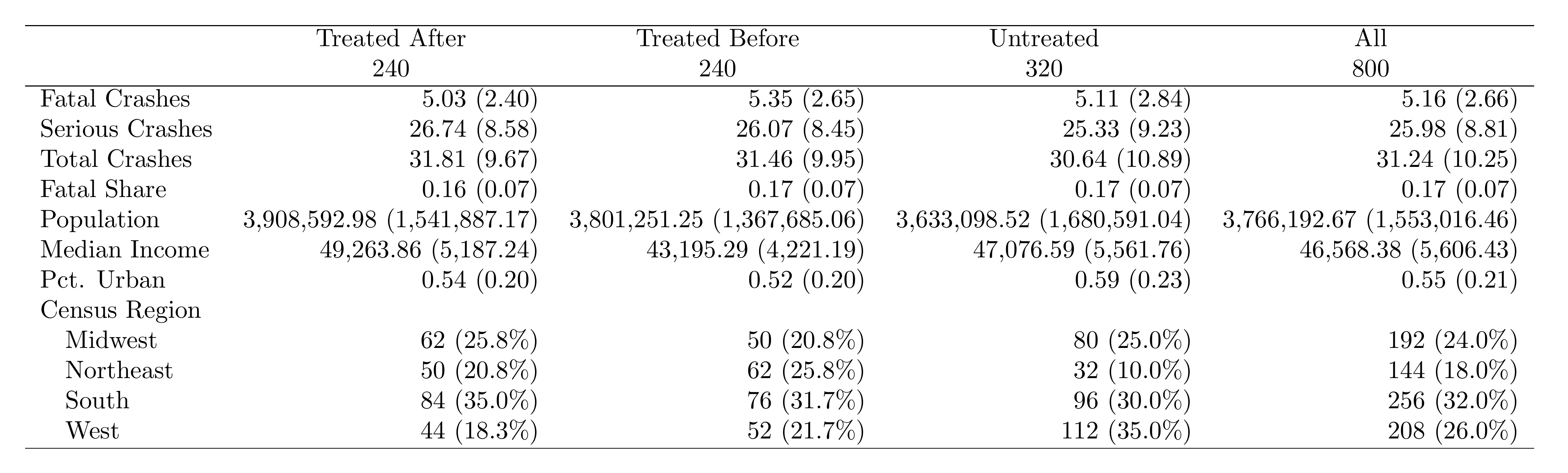
What to Look For

Pre-treatment balance: Treated Before vs. Untreated should look similar. Big differences suggest selection into treatment.
Post-treatment changes: Compare Treated After vs. Treated Before. This is the raw before/after for treated units.
Sample composition: Report observation counts for each group at the bottom of the table.

From Code Output to Publication-Ready Table

The code above produces a .tex file containing the table body. To get a publication-ready PDF, wrap it in a standalone LaTeX document and compile:

\documentclass[border=10pt]{standalone}
\usepackage{booktabs}
\begin{document}
\input{descriptive_table.tex}
\end{document}

Compile with pdflatex standalone_table.tex. See the LaTeX module for installation details.

Table Formatting Checklist

Use booktabs rules (\toprule, \midrule, \bottomrule) — never vertical lines or heavy grids
Standard errors in parentheses directly below coefficients
Stars for significance with a clear legend at the bottom
Round consistently: 2-3 decimal places for coefficients, 3 for standard errors
Label variables clearly: "Log(Population)" not "log_pop"
Fixed effects indicators: "Yes" or blank (not "No")
Sample size and R-squared at the bottom of every regression table

AI Tools Are Great for Table Formatting

Formatting tables and figures is an excellent use case for AI tools like ChatGPT or Claude. These tasks leave little room for hallucination—the AI just needs to adjust spacing, labels, and LaTeX formatting. Describe what you want and iterate.

Part E: Difference-in-Differences and Event Study

The TWFE Regression

With our merged panel, we estimate the effect of the policy on fatal crashes using two-way fixed effects (state + year FE):

$$ Y_{st} = \gamma_s + \delta_t + \beta \cdot (\text{Treat} \times \text{Post})_{st} + \varepsilon_{st} $$

where $\gamma_s$ are state fixed effects, $\delta_t$ are year fixed effects, and $\beta$ is the treatment effect.

use "$build/output/analysis_panel.dta", clear

* Create log outcome
gen log_fatal = log(fatal_crashes + 1)

* Label variables for table output
label variable post_treated "Post × Treated"
label variable log_pop "Log Population"
label variable median_income "Median Income"

* Main DD regression: effect of policy on log fatal crashes
reghdfe log_fatal post_treated, absorb(state_fips year) vce(cluster state_fips)

pacman::p_load(fixest, data.table)

panel <- fread("build/output/analysis_panel.csv")
panel[, log_fatal := log(fatal_crashes + 1)]

# Main DD regression
main <- feols(
  log_fatal ~ post_treated | state_fips + year,
  data = panel, vcov = ~state_fips
)
summary(main)

import pyfixest as pf
import pandas as pd
import numpy as np

panel = pd.read_csv("build/output/analysis_panel.csv")
panel['log_fatal'] = np.log(panel['fatal_crashes'] + 1)

# Main DD regression
main = pf.feols(
    "log_fatal ~ post_treated | state_fips + year",
    vcov={"CRV1": "state_fips"}, data=panel
)
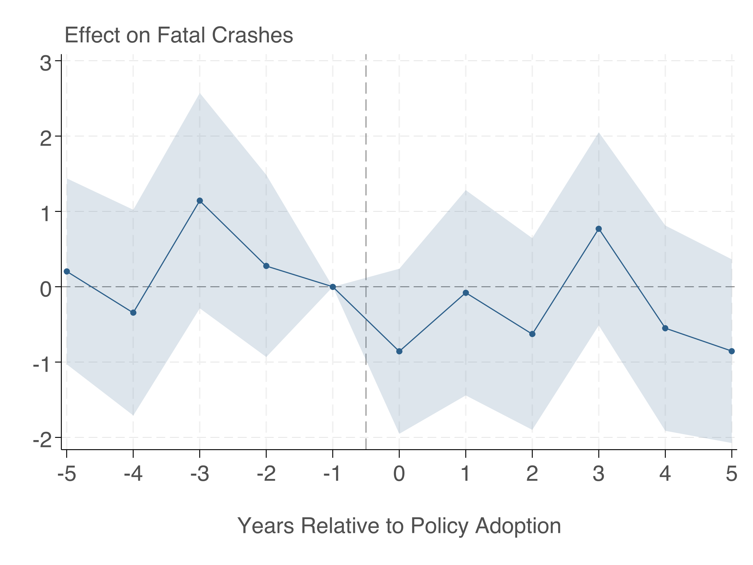
main.summary()

Event Study

The event study shows dynamic treatment effects and lets us check the parallel trends assumption.

use "$build/output/analysis_panel.dta", clear

* Create time-to-treatment (never-treated get a far-away value)
gen time_to_treat = year - adoption_year
replace time_to_treat = -99 if missing(adoption_year)

* Create dummies: rel_m5 ... rel_m1, rel_0 ... rel_5
forvalues t = -5/5 {
    if `t' < 0 {
        local name "m`= abs(`t')'"
    }
    else {
        local name "`t'"
    }
    gen rel_`name' = (time_to_treat == `t')
}

* Bin endpoints
replace rel_m5 = (time_to_treat <= -5) & !missing(adoption_year)
replace rel_5  = (time_to_treat >= 5)  & !missing(adoption_year)

* Create log outcome
gen log_fatal = log(fatal_crashes + 1)

* Regression (omit t=-1)
reghdfe log_fatal rel_m5 rel_m4 rel_m3 rel_m2 ///
    rel_0 rel_1 rel_2 rel_3 rel_4 rel_5 log_pop, ///
    absorb(state_fips year) vce(cluster state_fips)

estimates store event_study

* Extract coefficients and SEs into matrices
matrix b = e(b)
matrix V = e(V)

preserve
clear
set obs 11
gen t = .
gen coef = .
gen se = .

local coefs "rel_m5 rel_m4 rel_m3 rel_m2 rel_0 rel_1 rel_2 rel_3 rel_4 rel_5"
local i = 1
foreach v of local coefs {
    if `i' <= 4 { replace t = `i' - 6 in `i' }
    else        { replace t = `i' - 5 in `i' }
    replace coef = b[1, `i'] in `i'
    replace se = sqrt(V[`i', `i']) in `i'
    local i = `i' + 1
}

* Add omitted period (t = -1, coefficient = 0)
replace t = -1 in 11
replace coef = 0 in 11
replace se = 0 in 11

gen ub = coef + 1.96 * se
gen lb = coef - 1.96 * se
sort t

* Shaded confidence bands (ribbons) + connected points
twoway (rarea ub lb t, color("44 95 138%20") lwidth(none)) ///
       (connected coef t, mcolor("44 95 138") lcolor("44 95 138") ///
            msize(small) msymbol(O) lwidth(medthin)), ///
    yline(0, lcolor(gs8) lwidth(thin)) ///
    xline(-0.5, lcolor(gs8) lwidth(thin) lpattern(dash)) ///
    xtitle("Years Relative to Policy Adoption", ///
           size(large) margin(t=3) color(gs5)) ///
    ytitle("") ///
    ylabel(, labsize(large) labcolor(gs5) grid glcolor(gs14) glwidth(vthin)) ///
    xlabel(-5(1)5, labsize(large) labcolor(gs5)) ///
    title("Effect on Log Fatal Crashes", ///
          position(11) size(large) color(gs5)) ///
    legend(off) ///
    graphregion(color(white) margin(medium)) ///
    plotregion(color(white) margin(small))

graph export "$analysis/output/figures/event_study.png", replace width(2400) height(1800)
restore

pacman::p_load(fixest, ggfixest, data.table)

panel <- fread("build/output/analysis_panel.csv")
panel[, log_fatal := log(fatal_crashes + 1)]

# Create time-to-treatment
# Never-treated: set to -1000
panel[, time_to_treat := fifelse(
  is.na(adoption_year), -1000L,
  as.integer(year - adoption_year)
)]
panel[, ever_treated := fifelse(!is.na(adoption_year), 1L, 0L)]

# Bin endpoints
panel[, time_to_treat := fifelse(
  time_to_treat == -1000, -1000L,
  as.integer(pmax(-5, pmin(5, time_to_treat)))
)]

# Event study regression
es <- feols(
  log_fatal ~ i(time_to_treat, ever_treated,
                     ref = c(-1, -1000)) + log_pop
    | state_fips + year,
  data = panel, vcov = ~state_fips
)
summary(es)

# Plot
ggiplot(es) +
  labs(x = "Years Relative to Policy Adoption",
       y = "Effect on Log Fatal Crashes") +
  geom_hline(yintercept = 0, linetype = "dashed") +
  theme_minimal()
ggsave("analysis/output/figures/event_study.png", width = 8, height = 5, dpi = 300)

import pyfixest as pf
import pandas as pd
import numpy as np

panel = pd.read_csv("build/output/analysis_panel.csv")
panel['log_fatal'] = np.log(panel['fatal_crashes'] + 1)

# Create time-to-treatment
panel['time_to_treat'] = panel['year'] - panel['adoption_year']
panel['time_to_treat'] = panel['time_to_treat'].fillna(-1000).astype(int)
panel['ever_treated'] = panel['adoption_year'].notna().astype(int)

# Bin endpoints
panel['time_to_treat'] = np.where(
    panel['time_to_treat'] == -1000, -1000,
    np.clip(panel['time_to_treat'], -5, 5)
)

# Event study regression
es = pf.feols(
    "log_fatal ~ i(time_to_treat, ever_treated, ref=c(-1, -1000))"
    " + log_pop | state_fips + year",
    vcov={"CRV1": "state_fips"}, data=panel
)
es.summary()

# Plot
es.iplot()

Here's the event study plot produced by the Stata code above:

Making Figures Publication-Ready

Stata's default graphs look terrible. With a few tweaks, you can produce figures that look like they belong in a top journal. The key reference is Schwabish (2014), "An Economist's Guide to Visualizing Data" (JEP). Tal Gross has an excellent thread showing exactly how to transform Stata's defaults into clean, publication-quality output:

Make your graphs better in three easy steps…
— Tal Gross (@talgross.bsky.social) March 11, 2025

To start, here's a graph with the default Stata options.
— Tal Gross (@talgross.bsky.social) March 11, 2025

Step 1: labels not legends. This makes the graph much easier to read.
— Tal Gross (@talgross.bsky.social) March 11, 2025

Step 2: all text horizontal. Horizontal text is easier to read than vertical text.
— Tal Gross (@talgross.bsky.social) March 11, 2025

Step 3: eliminated unnecessary ink.
— Tal Gross (@talgross.bsky.social) March 11, 2025

That's Stata, here's a start in R.
— Tal Gross (@talgross.bsky.social) March 11, 2025

The event study plot above follows these principles. Here's a summary of the key steps:

Remove clutter. No top/right borders (graphregion(color(white))), no unnecessary gridlines, no legend when you can label directly.
Use a single accent color for your main result. Use gray for reference lines and context. The code above uses mcolor("44 95 138") — a muted blue.
Shaded confidence bands are cleaner than error bars for continuous data. In Stata, use rarea for shaded bands instead of rcap for error bars. The event study code above demonstrates this — the twoway rarea command creates the shaded CI bands, while connected plots the point estimates.
Informative axis labels. "Years Relative to Policy Adoption" not "period". Use xtitle() and ytitle() with readable sizes.
Remove the plot title. Economics papers put the title in the figure caption, not on the plot itself.
Export at high resolution. Use graph export "file.png", width(2400) or export as PDF for vector graphics.

Figure Checklist

Can you read all text when the figure is printed at its final size?
Are axis labels descriptive? (not variable names)
Is the aspect ratio wider than tall? (roughly 4:3 or 16:10)
Is the resolution at least 300 DPI for print?
Did you export as PDF (vector) or high-res PNG?
Is the background white? (no gray default)
Are confidence intervals shown as shaded bands (not error bars) where appropriate?

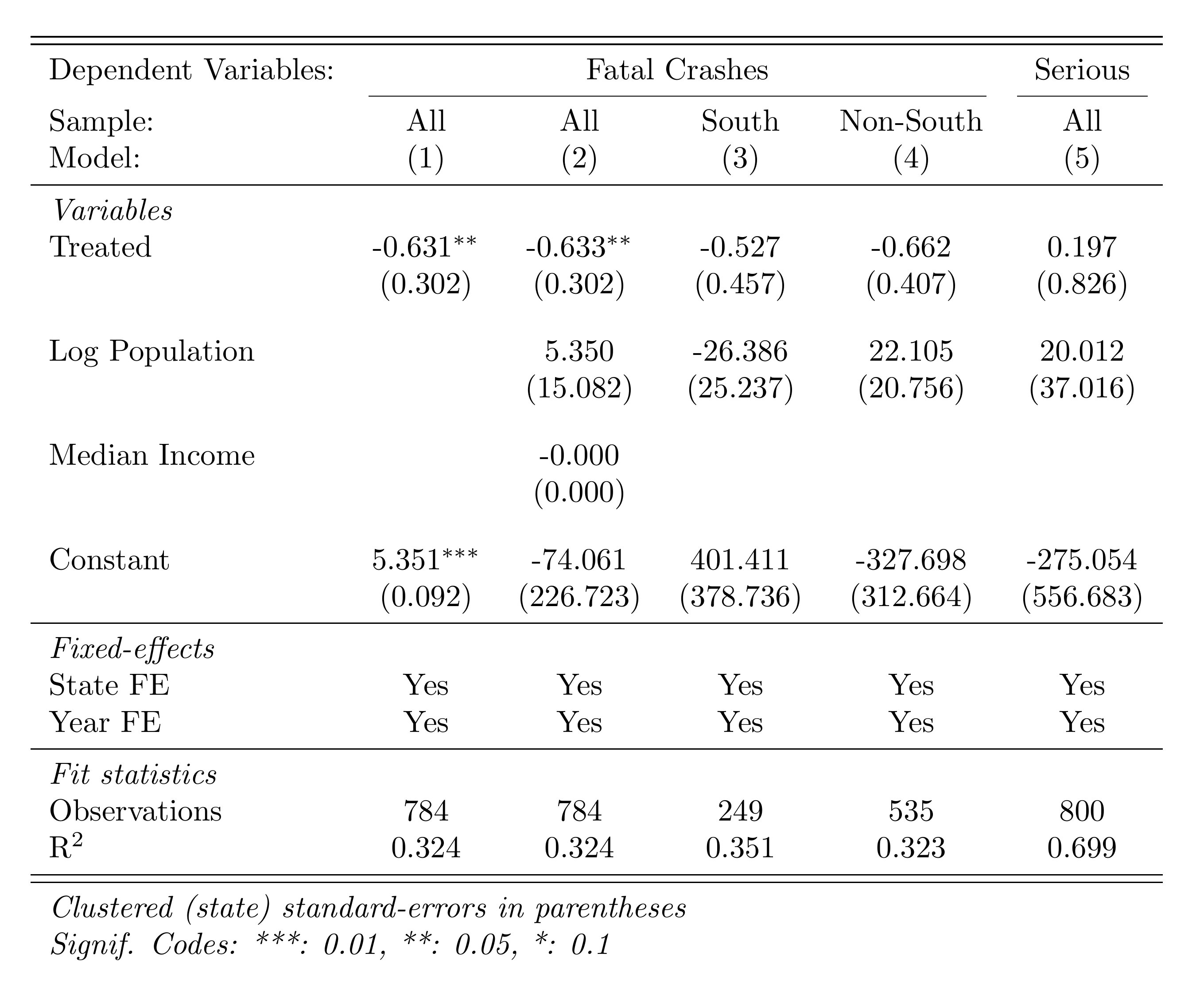
Part F: Professional DD Table with Subgroups

A strong empirical paper doesn't just report the main result. It shows robustness across specifications and explores heterogeneity. Here we create a single table with: (1) the main result, (2) results by region subgroup, and (3) a specification with additional controls.

use "$build/output/analysis_panel.dta", clear

* Label variables for table output
label variable post_treated "Post × Treated"
label variable log_pop "Log Population"
label variable median_income "Median Income"

* Col 1: Main result
reghdfe fatal_crashes post_treated, absorb(state_fips year) vce(cluster state_fips)
estadd local state_fe "Yes"
estadd local year_fe "Yes"
estimates store m1

* Col 2: With controls
reghdfe fatal_crashes post_treated log_pop median_income, ///
    absorb(state_fips year) vce(cluster state_fips)
estadd local state_fe "Yes"
estadd local year_fe "Yes"
estimates store m2

* Col 3: South only
reghdfe fatal_crashes post_treated log_pop if region == "South", ///
    absorb(state_fips year) vce(cluster state_fips)
estadd local state_fe "Yes"
estadd local year_fe "Yes"
estimates store m3

* Col 4: Non-South
reghdfe fatal_crashes post_treated log_pop if region != "South", ///
    absorb(state_fips year) vce(cluster state_fips)
estadd local state_fe "Yes"
estadd local year_fe "Yes"
estimates store m4

* Col 5: Serious crashes as outcome
reghdfe serious_crashes post_treated log_pop, ///
    absorb(state_fips year) vce(cluster state_fips)
estadd local state_fe "Yes"
estadd local year_fe "Yes"
estimates store m5

* Export professional table
esttab m1 m2 m3 m4 m5 ///
    using "$analysis/output/tables/dd_results.tex", replace ///
    se(%9.3f) b(%9.3f) ///
    star(* 0.10 ** 0.05 *** 0.01) ///
    nomtitles nonumbers ///
    label fragment ///
    prehead("\begin{tabular}{l*{5}{c}}" ///
            "\midrule \midrule" ///
            "Dependent Variables: &\multicolumn{4}{c}{Fatal Crashes} &Serious\\" ///
            "\cmidrule(lr){2-5} \cmidrule(lr){6-6}" ///
            "Sample: & All & All & South & Non-South & All \\" ///
            "Model: & (1) & (2) & (3) & (4) & (5) \\" ///
            "\midrule" ///
            "\emph{Variables} \\") ///
    posthead("") ///
    prefoot("\midrule" ///
            "\emph{Fixed-effects} \\") ///
    stats(state_fe year_fe N r2, ///
        labels("State FE" "Year FE" ///
               "\midrule \emph{Fit statistics} \\ Observations" ///
               "R\$^2\$") ///
        fmt(%s %s %9.0fc %9.3f)) ///
    postfoot("\midrule \midrule" ///
             "\multicolumn{6}{l}{\emph{Clustered (state) standard-errors in parentheses}}\\" ///
             "\multicolumn{6}{l}{\emph{Signif. Codes: ***: 0.01, **: 0.05, *: 0.1}}\\" ///
             "\end{tabular}")

pacman::p_load(fixest, data.table)

panel <- fread("build/output/analysis_panel.csv")

# Col 1: Main result
m1 <- feols(fatal_crashes ~ post_treated | state_fips + year,
            data = panel, vcov = ~state_fips)

# Col 2: With controls
m2 <- feols(fatal_crashes ~ post_treated + log_pop + median_income
            | state_fips + year,
            data = panel, vcov = ~state_fips)

# Col 3: South only
m3 <- feols(fatal_crashes ~ post_treated + log_pop | state_fips + year,
            data = panel[region == "South"], vcov = ~state_fips)

# Col 4: Non-South
m4 <- feols(fatal_crashes ~ post_treated + log_pop | state_fips + year,
            data = panel[region != "South"], vcov = ~state_fips)

# Col 5: Serious crashes as outcome
m5 <- feols(serious_crashes ~ post_treated + log_pop | state_fips + year,
            data = panel, vcov = ~state_fips)

# Export professional table
etable(
  m1, m2, m3, m4, m5,
  tex = TRUE, file = "analysis/output/tables/dd_table.tex", replace = TRUE,
  headers = list(
    ":_sym:" = c("(1)", "(2)", "(3)", "(4)", "(5)")
  ),
  style.tex = style.tex(
    depvar.title = "Dep. Var.:",
    fixef.title = "\\midrule",
    yesNo = c("Yes", ""),
    stats.title = "\\midrule"
  ),
  fitstat = ~ n + r2 + wr2,
  dict = c(
    fatal_crashes = "Fatal Crashes",
    serious_crashes = "Serious Crashes",
    post_treated = "Post × Treated",
    log_pop = "Log(Population)",
    median_income = "Median Income"
  ),
  se.below = TRUE, depvar = TRUE
)

import pyfixest as pf
import pandas as pd

panel = pd.read_csv("build/output/analysis_panel.csv")

# Col 1: Main result
m1 = pf.feols("fatal_crashes ~ post_treated | state_fips + year",
              vcov={"CRV1": "state_fips"}, data=panel)

# Col 2: With controls
m2 = pf.feols("fatal_crashes ~ post_treated + log_pop + median_income"
              " | state_fips + year",
              vcov={"CRV1": "state_fips"}, data=panel)

# Col 3: South only
m3 = pf.feols("fatal_crashes ~ post_treated + log_pop | state_fips + year",
              vcov={"CRV1": "state_fips"},
              data=panel[panel['region'] == 'South'])

# Col 4: Non-South
m4 = pf.feols("fatal_crashes ~ post_treated + log_pop | state_fips + year",
              vcov={"CRV1": "state_fips"},
              data=panel[panel['region'] != 'South'])

# Col 5: Serious crashes as outcome
m5 = pf.feols("serious_crashes ~ post_treated + log_pop | state_fips + year",
              vcov={"CRV1": "state_fips"}, data=panel)

# Export table
pf.etable(
    [m1, m2, m3, m4, m5],
    type="tex",
    file="analysis/output/tables/dd_table.tex",
    labels={
        "fatal_crashes": "Fatal Crashes",
        "serious_crashes": "Serious Crashes",
        "post_treated": "Post × Treated",
        "log_pop": "Log(Population)",
        "median_income": "Median Income",
    },
)

Here's the DD regression table produced by esttab:

Part G: Instrumental Variables

This section uses a separate, pre-built dataset (iv_data.csv) inspired by Angrist & Lavy (1999). We estimate the effect of class size on test scores, using a Maimonides-rule instrument (enrollment determines class size via a maximum-of-40 rule).

The Setup

Endogenous variable: class_size (correlated with school quality)
Instrument: enrollment (determines class size via the Maimonides rule, but plausibly doesn't directly affect test scores)
Outcome: test_score

The three IV equations:

First stage: $ D_i = \alpha_0 + \alpha_1 Z_i + \alpha_2 X_i + \nu_i $

Reduced form: $ Y_i = \pi_0 + \pi_1 Z_i + \pi_2 X_i + \eta_i $

2SLS (structural): $ Y_i = \beta_0 + \beta_1 D_i + \beta_2 X_i + \varepsilon_i $

where $Y_i$ is test score, $D_i$ is class size (endogenous), $Z_i$ is enrollment (instrument), and $X_i$ are controls. The IV estimate is $\hat{\beta}_1 = \hat{\pi}_1 / \hat{\alpha}_1$.

First Stage

Does the instrument predict the endogenous variable? Check the F-statistic — it should be well above 10.

import delimited "$analysis/code/iv_data.csv", clear

* Label variables
label variable class_size "Class Size"
label variable test_score "Test Score"
label variable enrollment "Enrollment"
label variable pct_disadvantaged "Pct. Disadvantaged"

* First stage: Does enrollment predict class size?
regress class_size enrollment pct_disadvantaged, vce(robust)
estimates store first_stage

* Check the F-stat on enrollment — should be >> 10
test enrollment

pacman::p_load(fixest, data.table)

iv_data <- fread("analysis/code/iv_data.csv")

# First stage: Does enrollment predict class size?
first_stage <- feols(class_size ~ enrollment + pct_disadvantaged,
                     data = iv_data)
summary(first_stage)

# F-statistic on excluded instrument
cat("First-stage F:", fitstat(first_stage, "f")$f$stat, "\n")

import pandas as pd
import pyfixest as pf

iv_data = pd.read_csv("analysis/code/iv_data.csv")

# First stage: Does enrollment predict class size?
first_stage = pf.feols(
    "class_size ~ enrollment + pct_disadvantaged",
    data=iv_data, vcov="hetero"
)
first_stage.summary()

# F-statistic on excluded instrument
enrollment_coef = first_stage.coef()['enrollment']
enrollment_se = first_stage.se()['enrollment']
f_stat = (enrollment_coef / enrollment_se) ** 2
print(f"\nFirst-stage F-statistic: {f_stat:.1f}")

Reduced Form

The reduced form regresses the outcome directly on the instrument. If the instrument affects the outcome, it's working through the endogenous variable.

* Reduced form: Does enrollment predict test scores?
regress test_score enrollment pct_disadvantaged, vce(robust)
estimates store reduced_form

# Reduced form: Does enrollment predict test scores?
reduced_form <- feols(test_score ~ enrollment + pct_disadvantaged,
                      data = iv_data)
summary(reduced_form)

# Reduced form: Does enrollment predict test scores?
reduced_form = pf.feols(
    "test_score ~ enrollment + pct_disadvantaged",
    data=iv_data, vcov="hetero"
)
reduced_form.summary()

2SLS Estimation

* OLS (biased estimate)
regress test_score class_size pct_disadvantaged, vce(robust)
estimates store ols

* 2SLS: Instrument class_size with enrollment
ivregress 2sls test_score pct_disadvantaged (class_size = enrollment), ///
    vce(robust) first
estimates store iv_2sls

* Export all four specifications
esttab first_stage reduced_form iv_2sls ols ///
    using "$analysis/output/tables/iv_results.tex", replace ///
    label fragment ///
    order(class_size enrollment pct_disadvantaged) ///
    b(%9.3f) se(%9.3f) ///
    star(* 0.10 ** 0.05 *** 0.01) ///
    nomtitles nonumbers ///
    prehead("\begin{tabular}{l*{4}{c}}" ///
            "\midrule \midrule" ///
            "Dependent Variable: & Class Size & \multicolumn{3}{c}{Test Score}\\" ///
            "\cmidrule(lr){2-2} \cmidrule(lr){3-5}" ///
            "Model: & First Stage & Reduced Form & 2SLS & OLS\\" ///
            "& (1) & (2) & (3) & (4)\\" ///
            "\midrule" ///
            "\emph{Variables} \\") ///
    posthead("") ///
    prefoot("\midrule" ///
            "\emph{Fit statistics} \\") ///
    stats(N r2, fmt(%9.0fc %9.3f) ///
          labels("Observations" "R\$^2\$")) ///
    postfoot("\midrule \midrule" ///
             "\multicolumn{5}{l}{\emph{Heteroskedasticity-robust standard-errors in parentheses}}\\" ///
             "\multicolumn{5}{l}{\emph{Instrument: School enrollment}}\\" ///
             "\multicolumn{5}{l}{\emph{Signif. Codes: ***: 0.01, **: 0.05, *: 0.1}}\\" ///
             "\end{tabular}")

# 2SLS: Instrument class_size with enrollment
# fixest syntax: outcome ~ controls | FE | endogenous ~ instrument
iv_model <- feols(
  test_score ~ pct_disadvantaged | 0 | class_size ~ enrollment,
  data = iv_data
)
summary(iv_model)

# First-stage F
cat("First-stage F:", fitstat(iv_model, "ivf")$ivf$stat, "\n")

# Compare OLS vs IV
ols_model <- feols(test_score ~ class_size + pct_disadvantaged,
                   data = iv_data)
etable(ols_model, iv_model,
       dict = c(class_size = "Class Size",
                fit_class_size = "Class Size (IV)"))

import pyfixest as pf

# 2SLS: Instrument class_size with enrollment
iv_model = pf.feols(
    "test_score ~ pct_disadvantaged | 0 | class_size ~ enrollment",
    data=iv_data, vcov="hetero"
)
iv_model.summary()

# Compare: OLS
ols_model = pf.feols(
    "test_score ~ class_size + pct_disadvantaged",
    data=iv_data, vcov="hetero"
)

# Compare coefficients
print(f"\nOLS class_size coef: {ols_model.coef()['class_size']:.3f}")
print(f"IV  class_size coef: {iv_model.coef()['class_size']:.3f}")

Here's the IV results table comparing OLS, first stage, reduced form, and 2SLS:

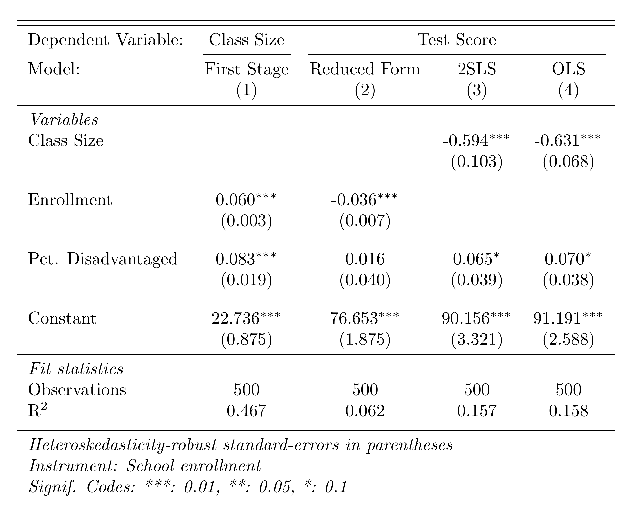
OLS vs. IV: What to Expect

OLS is biased because class size is correlated with school quality (omitted variable bias). The IV estimate isolates the causal effect by using only variation in class size driven by enrollment thresholds. The IV estimate should typically be larger in magnitude if OLS is biased toward zero (attenuation bias from measurement error) or could go either way depending on the source of endogeneity.

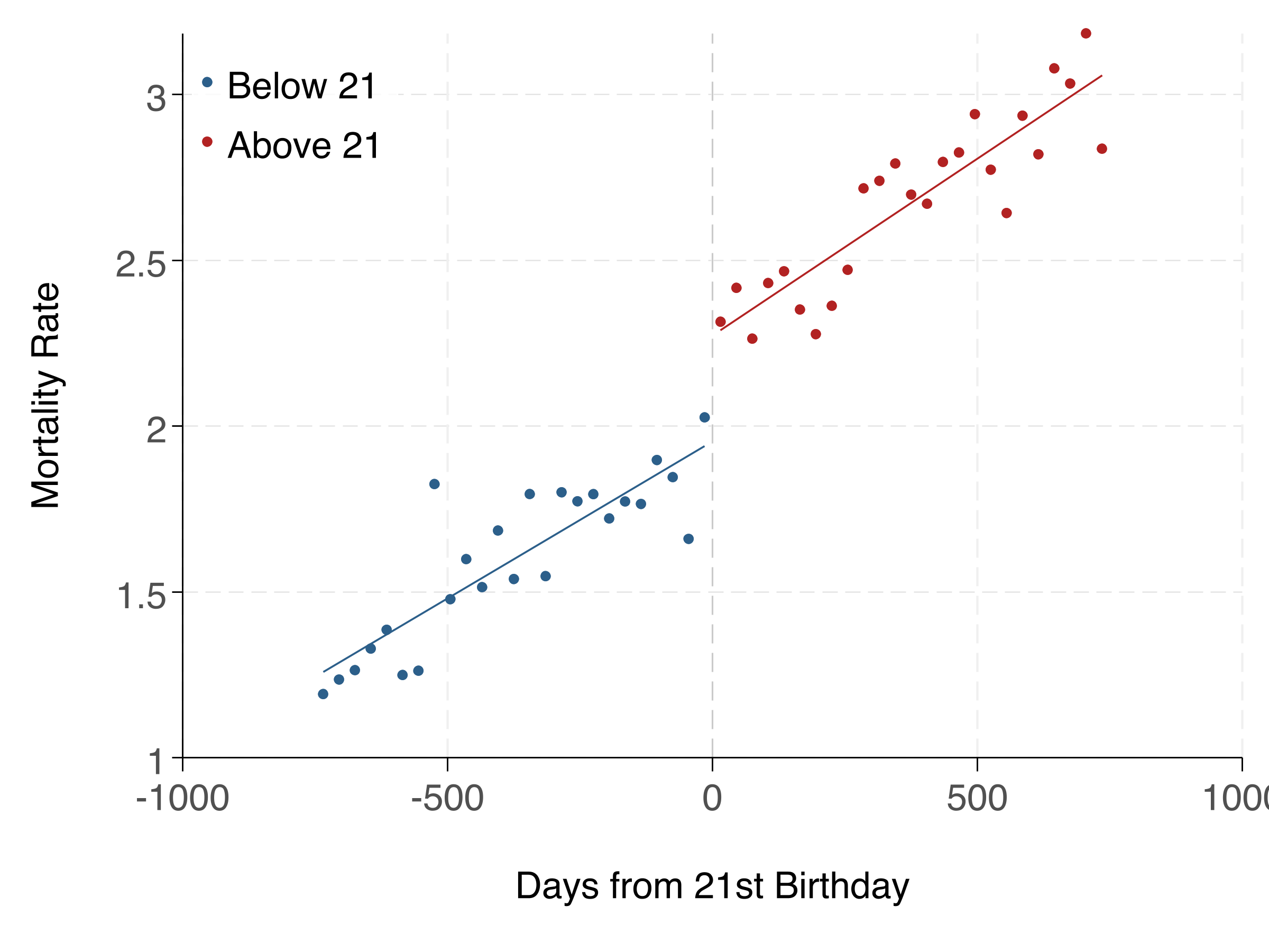
Part H: Regression Discontinuity

This section uses a pre-built dataset (rd_data.csv) inspired by Carpenter & Dobkin (2009). We estimate the effect of legal drinking access (turning 21) on mortality using a sharp RD design.

The Setup

Running variable: days_from_21 (days relative to 21st birthday)
Cutoff: 0 (turning 21)
Treatment: over_21 (legal access to alcohol)
Outcome: mortality_rate

The RD estimating equation (linear specification):

$$ Y_i = \alpha + \tau \cdot \mathbf{1}[X_i \geq c] + \beta_1 (X_i - c) + \beta_2 (X_i - c) \cdot \mathbf{1}[X_i \geq c] + \varepsilon_i $$

where $X_i$ is the running variable (days from 21), $c = 0$ is the cutoff, and $\tau$ is the treatment effect — the jump in mortality at age 21.

Linear Specification

The simplest RD: a linear function of the running variable on each side of the cutoff, within a bandwidth.

import delimited "$analysis/code/rd_data.csv", clear

* Label variables
label variable mortality_rate "Mortality Rate"
label variable over_21 "Over 21"
label variable days_from_21 "Days from 21st Birthday"

* Create interaction term
gen days_x_over21 = days_from_21 * over_21

* Linear RD within bandwidth of 365 days
regress mortality_rate over_21 days_from_21 days_x_over21 ///
    if abs(days_from_21) <= 365, vce(robust)
estimates store rd_linear

* The coefficient on over_21 is the RD estimate (jump at cutoff)

pacman::p_load(fixest, data.table)

rd_data <- fread("analysis/code/rd_data.csv")

# Linear RD within bandwidth of 365 days
rd_linear <- feols(
  mortality_rate ~ over_21 + days_from_21 + over_21:days_from_21,
  data = rd_data[abs(days_from_21) <= 365]
)
summary(rd_linear)

# Narrower bandwidth (180 days)
rd_narrow <- feols(
  mortality_rate ~ over_21 + days_from_21 + over_21:days_from_21,
  data = rd_data[abs(days_from_21) <= 180]
)
summary(rd_narrow)

import pandas as pd
import pyfixest as pf

rd_data = pd.read_csv("analysis/code/rd_data.csv")

# Linear RD within bandwidth of 365 days
subset = rd_data[rd_data['days_from_21'].abs() <= 365].copy()
rd_linear = pf.feols(
    'mortality_rate ~ over_21 + days_from_21 + over_21:days_from_21',
    data=subset, vcov="hetero"
)
print("=== Linear RD (bw=365) ===")
rd_linear.summary()

# Narrower bandwidth (180 days)
subset_narrow = rd_data[rd_data['days_from_21'].abs() <= 180].copy()
rd_narrow = pf.feols(
    'mortality_rate ~ over_21 + days_from_21 + over_21:days_from_21',
    data=subset_narrow, vcov="hetero"
)
print("\n=== Linear RD (bw=180) ===")
rd_narrow.summary()

Polynomial Specification

A polynomial specification allows for curvature in the relationship between the running variable and the outcome. This can be more flexible but risks overfitting.

* Create polynomial terms
gen days_sq = days_from_21^2
gen days_cu = days_from_21^3
gen days_sq_x_over21 = days_sq * over_21
gen days_cu_x_over21 = days_cu * over_21

* Quadratic RD
regress mortality_rate over_21 days_from_21 days_x_over21 ///
    days_sq days_sq_x_over21 ///
    if abs(days_from_21) <= 365, vce(robust)
estimates store rd_quadratic

* Cubic RD
regress mortality_rate over_21 days_from_21 days_x_over21 ///
    days_sq days_sq_x_over21 days_cu days_cu_x_over21 ///
    if abs(days_from_21) <= 365, vce(robust)
estimates store rd_cubic

* Export results table
esttab rd_linear rd_quadratic rd_cubic ///
    using "$analysis/output/tables/rd_results.tex", replace ///
    keep(over_21) label fragment ///
    b(%9.4f) se(%9.4f) ///
    star(* 0.10 ** 0.05 *** 0.01) ///
    nomtitles nonumbers ///
    prehead("\begin{tabular}{l*{3}{c}}" ///
            "\midrule \midrule" ///
            "Dependent Variable: &\multicolumn{3}{c}{Mortality Rate}\\" ///
            "\cmidrule(lr){2-4}" ///
            "Model:              & Linear & Quadratic & Cubic\\" ///
            "                    & (1) & (2) & (3)\\" ///
            "\midrule" ///
            "\emph{Variables} \\") ///
    posthead("") ///
    prefoot("\midrule" ///
            "\emph{Fit statistics} \\") ///
    stats(N r2, fmt(%9.0fc %9.4f) ///
          labels("Observations" "R\$^2\$")) ///
    postfoot("\midrule \midrule" ///
             "\multicolumn{4}{l}{\emph{Robust standard-errors in parentheses}}\\" ///
             "\multicolumn{4}{l}{\emph{Signif. Codes: ***: 0.01, **: 0.05, *: 0.1}}\\" ///
             "\end{tabular}")

pacman::p_load(fixest, rdrobust, data.table)

rd_data <- fread("analysis/code/rd_data.csv")

# Quadratic RD
rd_data[, days2 := days_from_21^2]
rd_quad <- feols(
  mortality_rate ~ over_21 + days_from_21 + days2 +
    over_21:days_from_21 + over_21:days2,
  data = rd_data[abs(days_from_21) <= 365]
)
summary(rd_quad)

# Using rdrobust for optimal bandwidth selection
rd_robust <- rdrobust(
  y = rd_data$mortality_rate,
  x = rd_data$days_from_21,
  c = 0
)
summary(rd_robust)

# RD plot
rdplot(
  y = rd_data$mortality_rate,
  x = rd_data$days_from_21,
  c = 0,
  title = "RD Plot: Mortality at Age 21",
  x.label = "Days from 21st Birthday",
  y.label = "Mortality Rate"
)

import numpy as np
import matplotlib.pyplot as plt
import pandas as pd
import pyfixest as pf

rd_data = pd.read_csv("analysis/code/rd_data.csv")

# Quadratic RD
rd_data['days2'] = rd_data['days_from_21'] ** 2
subset = rd_data[rd_data['days_from_21'].abs() <= 365].copy()
rd_quad = pf.feols(
    'mortality_rate ~ over_21 + days_from_21 + days2'
    ' + over_21:days_from_21 + over_21:days2',
    data=subset, vcov="hetero"
)
print("=== Quadratic RD ===")
rd_quad.summary()

# RD Plot
fig, ax = plt.subplots(figsize=(8, 5))
# Bin the data
bins = np.arange(-365, 366, 30)
rd_data['bin'] = pd.cut(rd_data['days_from_21'], bins=bins)
binned = rd_data.groupby('bin')['mortality_rate'].mean().reset_index()
binned['mid'] = binned['bin'].apply(lambda x: x.mid if pd.notna(x) else np.nan)
binned = binned.dropna()

ax.scatter(binned['mid'], binned['mortality_rate'], s=20, alpha=0.7)
ax.axvline(0, color='red', linestyle='--', linewidth=0.8)
ax.set_xlabel('Days from 21st Birthday')
ax.set_ylabel('Mortality Rate')
ax.set_title('RD Plot: Mortality at Age 21')
ax.spines['top'].set_visible(False)
ax.spines['right'].set_visible(False)
fig.tight_layout()
fig.savefig('analysis/output/figures/rd_plot.png', dpi=300)

Here's the RD plot and regression table:

RD plot with linear fit showing a clear discontinuity in mortality at age 21.

RD plot with polynomial fit. The discontinuity is robust to allowing curvature in the running variable.

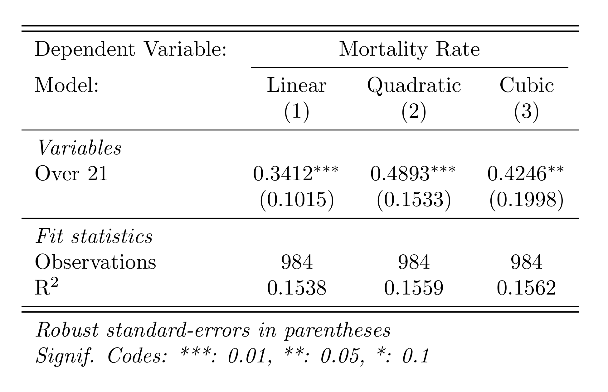
Linear vs. Polynomial: Which to Use?

Start with linear — it's simpler and less prone to overfitting. Use polynomial specifications as robustness checks. If the linear and polynomial estimates are very different, it suggests the result may be sensitive to functional form assumptions. The rdrobust package provides data-driven bandwidth selection and bias-corrected inference, and is the current best practice.

Next: Diff-in-Diff and Event Studies →

Found something unclear or have a suggestion? Email [email protected].

Complete Project Walkthrough

Project Setup

Download the Project

Running Your Scripts

What's Inside

Key Principles

The Master File

Part A: Cleaning the Crash Data

Step 1: Read and Filter Crashes

Step 2: Collapse to State-Year-Severity

Step 3: Reshape and Save

Why Save Intermediate Files?

Part B: Cleaning the Demographics Data

Why Loop and Append?

Step 4: Loop and Append Demographics

Step 5: Clean and Collapse Demographics

Why Destring Income?

Part C: Merging Multiple Datasets

Understanding Merge Types

The keep() Option in Stata

The Rule of Thumb

Always Check Your Merges

Part D: Descriptive Statistics Table

What to Look For

From Code Output to Publication-Ready Table

Table Formatting Checklist

AI Tools Are Great for Table Formatting

Part E: Difference-in-Differences and Event Study

The TWFE Regression

Event Study

Making Figures Publication-Ready

Figure Checklist

Part F: Professional DD Table with Subgroups

Part G: Instrumental Variables

The Setup

First Stage

Reduced Form

2SLS Estimation

OLS vs. IV: What to Expect

Part H: Regression Discontinuity

The Setup

Linear Specification

Polynomial Specification

Linear vs. Polynomial: Which to Use?

The `keep()` Option in Stata