Data Fundamentals
Load, clean, reshape, and merge your data
Data wrangling is 80% of the work
The glamorous part of empirical economics is running regressions. But most of your time will be spent cleaning, reshaping, and merging data. This is normal. Professional economists spend most of their coding time on data prep too. Once you get comfortable with these operations, the analysis becomes straightforward.
Think of Data as Excel Spreadsheets
The datasets we work with in Stata and R are just tables—exactly like Excel spreadsheets. Each row is an observation (a person, a country-year, a transaction), and each column is a variable (age, GDP, price). If you've used Excel, you already understand the basic structure. The difference is that instead of clicking and dragging, we write code to manipulate these tables—which makes our work reproducible and scalable to millions of rows.
Choosing Your Unit of Analysis
Before you write any code, ask yourself: What is one row in my final dataset? This is your unit of analysis, and it determines everything else.
Common Units of Analysis in Economics
- Individual — One row per person (survey data, experiments)
- Individual-year — One row per person per year (labor panels)
- State-year — One row per state per year (policy studies)
- Country-year — One row per country per year (macro/trade)
- Firm — One row per company (cross-sectional)
- Firm-quarter — One row per company per quarter (finance panels)
- Transaction — One row per purchase/event (high-frequency data)
Your research question determines your unit of analysis. Consider these examples:
Unit: State-year
Policy varies by state and year. Outcome (employment) is also measured at state-year level.
Unit: Individual-year
Track individuals over time in panel data (e.g., NLSY, PSID) to see how education affects earnings trajectories.
Unit: State-year
Policy (BAC limit) varies by state and year. Fatalities are counted per state-year.
Unit: Individual-month
Track each person's employment status over time after treatment.
The Data Rarely Comes at the Right Level
You'll often need to aggregate raw data to match your unit of analysis. For example:
- You want state-year data, but your raw data has one row per car crash. You need to count crashes per state-year.
- You want individual-level data, but you have multiple survey responses per person. You need to collapse to one row per person.
- You want firm-year data, but you have daily stock prices. You need to aggregate to annual averages.
The Aggregating Data section below shows how to do this.
Reading & Writing Files
Loading Data
The first step in any analysis is loading your data into memory. Different file formats require different commands:
* Load Stata dataset
use "data.dta", clear

* Load CSV file
import delimited "data.csv", clear

* Load Excel file
import excel "data.xlsx", sheet("Sheet1") firstrow clear
pacman::p_load(haven, readr, readxl)
# Load Stata dataset
data <- read_dta("data.dta")
# Load CSV file
data <- read_csv("data.csv")
# Load Excel file
data <- read_excel("data.xlsx", sheet = "Sheet1")import pandas as pd
# Load Stata dataset
data = pd.read_stata("data.dta")
# Load CSV file
data = pd.read_csv("data.csv")
# Load Excel file
data = pd.read_excel("data.xlsx", sheet_name="Sheet1")Loading Specific Variables or Observations
For large datasets, you can load only what you need:
* Load only specific variables
use income age education using "data.dta", clear

* Load only observations meeting a condition
use "data.dta" if year == 2020, clear

* Combine both
use income age using "data.dta" if state == "CA", clear
# Load specific columns from CSV
data <- read_csv("data.csv", col_select = c(income, age, education))
# Filter while reading (with data.table for large files)
pacman::p_load(data.table)
data <- fread("data.csv", select = c("income", "age"))[year == 2020]# Load specific columns
data = pd.read_csv("data.csv", usecols=["income", "age", "education"])
# Load and filter (for very large files, use chunks)
data = pd.read_stata("data.dta", columns=["income", "age"])
data = data[data["year"] == 2020]Saving Data
After cleaning or transforming your data, save it so you don't have to re-run everything next time:
* Save as Stata dataset
save "cleaned_data.dta", replace

* Export to CSV
export delimited "cleaned_data.csv", replace
# Save as Stata dataset
write_dta(data, "cleaned_data.dta")
# Export to CSV
write_csv(data, "cleaned_data.csv")# Save as Stata dataset
data.to_stata("cleaned_data.dta", write_index=False)
# Export to CSV
data.to_csv("cleaned_data.csv", index=False)Save Intermediate Files
Save your data after each major step with numbered prefixes. When something breaks at step 5, you can start from step 4 instead of re-running everything:
01_imported.dta02_cleaned.dta03_merged.dta
Getting Your Data: Best Practices
Before you can load data, you need to get it. How you acquire your data matters for reproducibility.
Never modify your original data files. Ever. If you need to clean or transform data, write code that reads the raw file and saves a new cleaned version. This way you can always trace back to the original source.
Download Programmatically When Possible
The best way to get data is to download it with code. This makes your entire pipeline reproducible—anyone can run your script and get the same data.
* Example: Download FARS data (fatal crash data from NHTSA)
* Each year's data is a separate zip file

local years "2000 2001 2002 2003 2004 2005"

foreach year of local years {
    * Download the zip file
    copy "https://static.nhtsa.gov/nhtsa/downloads/FARS/`year'/National/FARS`year'NationalCSV.zip" ///
         "data/raw/FARS`year'.zip", replace

    * Unzip it
    unzipfile "data/raw/FARS`year'.zip", replace
}

* Now you have reproducible data acquisition!
# Example: Download FARS data (fatal crash data from NHTSA)
pacman::p_load(tidyverse)
years <- 2000:2005
for (year in years) {
url <- glue::glue(
"https://static.nhtsa.gov/nhtsa/downloads/FARS/{year}/National/FARS{year}NationalCSV.zip"
)
destfile <- glue::glue("data/raw/FARS{year}.zip")
# Download
download.file(url, destfile, mode = "wb")
# Unzip
unzip(destfile, exdir = glue::glue("data/raw/FARS{year}"))
}
# Now you have reproducible data acquisition!# Example: Download FARS data (fatal crash data from NHTSA)
import requests
import zipfile
from pathlib import Path
years = range(2000, 2006)
for year in years:
url = f"https://static.nhtsa.gov/nhtsa/downloads/FARS/{year}/National/FARS{year}NationalCSV.zip"
zip_path = Path(f"data/raw/FARS{year}.zip")
# Download
response = requests.get(url)
zip_path.write_bytes(response.content)
# Unzip
with zipfile.ZipFile(zip_path, 'r') as z:
z.extractall(f"data/raw/FARS{year}")
# Now you have reproducible data acquisition!Why Programmatic Downloads Matter
- Reproducibility: Anyone can run your code and get the exact same data
- Documentation: The URL in your code shows exactly where the data came from
- Automation: Easy to update when new data is released
- Version control: Your git history shows when you downloaded the data
When You Can't Download Programmatically
Sometimes data requires manual download (login required, CAPTCHA, web forms). In these cases, document thoroughly:
# Data Sources

## FARS (Fatality Analysis Reporting System)
- **Source:** NHTSA
- **URL:** https://www.nhtsa.gov/research-data/fatality-analysis-reporting-system-fars
- **Downloaded:** 2026-02-04
- **Files:** FARS2000.zip through FARS2008.zip
- **Archive:** https://web.archive.org/web/20260204/https://www.nhtsa.gov/...

## State Policy Data
- **Source:** Alcohol Policy Information System (APIS)
- **URL:** https://alcoholpolicy.niaaa.nih.gov/
- **Downloaded:** 2026-02-04
- **Notes:** Required selecting "Blood Alcohol Concentration Limits"
  and exporting to CSV. See screenshots in docs/data_download/
Archive Your Sources with archive.org
Websites change. Data gets moved or deleted. Before you start a project, archive your data sources:
- Go to web.archive.org
- Paste the URL of your data source
- Click "Save Page" to create an archived version
- Save the archive URL in your DATA_SOURCES.md
This way, even if the original website disappears, you (and anyone replicating your work) can see exactly where your data came from.
For data that requires navigating a web interface, take screenshots of each step. Save them in a docs/data_download/ folder. Future you (and your replicators) will thank you.
Data Cleaning
Inspecting Your Data
Before doing anything else, look at your data. How many observations? What variables exist? Are there missing values? Any obvious errors? These commands give you a quick overview:
* Overview of dataset
describe

* Summary statistics
summarize

* First few rows
list in 1/10

* Check for missing values
misstable summarize

* Detailed info on specific variables
codebook income education
# Overview of dataset
str(data)
glimpse(data)
# Summary statistics
summary(data)
# First few rows
head(data, 10)
# Check for missing values
colSums(is.na(data))# Overview of dataset
data.info()
data.dtypes
# Summary statistics
data.describe()
# First few rows
data.head(10)
# Check for missing values
data.isna().sum()Creating and Modifying Variables
Most analysis requires creating new variables—transformations like log income, indicators like "high earner," or cleaning up invalid values. Here are the essential operations:
* Create new variable
gen log_income = log(income)

* Conditional assignment
gen high_earner = (income > 100000)

* Modify variable
replace age = . if age < 0

* Drop observations
drop if missing(income)

* Keep only certain variables
keep id income age
pacman::p_load(dplyr)
data <- data %>%
mutate(
# Create new variable
log_income = log(income),
# Conditional assignment
high_earner = income > 100000,
# Modify variable
age = if_else(age < 0, NA_real_, age)
) %>%
# Drop observations
filter(!is.na(income)) %>%
# Keep only certain variables
select(id, income, age)import numpy as np
# Create new variable
data["log_income"] = np.log(data["income"])
# Conditional assignment
data["high_earner"] = data["income"] > 100000
# Modify variable
data.loc[data["age"] < 0, "age"] = np.nan
# Drop observations
data = data.dropna(subset=["income"])
# Keep only certain variables
data = data[["id", "income", "age"]]Recoding Categorical Variables
Often you need to convert continuous variables into categories (age groups, education levels) or simplify existing categories. This is called recoding:
* Recode numeric values into categories
recode education (1/8 = 1 "Less than HS") ///
                 (9/11 = 2 "Some HS") ///
                 (12 = 3 "HS Graduate") ///
                 (13/15 = 4 "Some College") ///
                 (16/20 = 5 "College+"), gen(educ_cat)

* Simple recode
recode age (18/29 = 1) (30/49 = 2) (50/64 = 3) (65/100 = 4), gen(age_group)
data <- data %>%
mutate(
educ_cat = case_when(
education <= 8 ~ "Less than HS",
education <= 11 ~ "Some HS",
education == 12 ~ "HS Graduate",
education <= 15 ~ "Some College",
education >= 16 ~ "College+"
),
age_group = cut(age, breaks = c(18, 30, 50, 65, 100),
labels = c("18-29", "30-49", "50-64", "65+"),
right = FALSE)
)# Using pd.cut for numeric ranges
data["age_group"] = pd.cut(data["age"],
bins=[18, 30, 50, 65, 100],
labels=["18-29", "30-49", "50-64", "65+"])
# Using np.select for complex recoding
conditions = [
data["education"] <= 8,
data["education"] <= 11,
data["education"] == 12,
data["education"] <= 15,
data["education"] >= 16
]
choices = ["Less than HS", "Some HS", "HS Graduate", "Some College", "College+"]
# Note: default="" required for numpy 1.25+ when choices are strings
data["educ_cat"] = np.select(conditions, choices, default="")Reshaping Data
Long Data is (Almost) Always Better
Most commands expect long format: multiple rows per unit, one column for values. If you're copy-pasting variable names with years (income_2018, income_2019...), you probably need to reshape to long.
Wide vs. Long Format
id  income_2020  income_2021
1   50000        52000
2   60000        61000
One row per unit. Each time period is a separate column.
id  year  income
1   2020  50000
1   2021  52000
2   2020  60000
2   2021  61000
Multiple rows per unit. Two columns (id + year) together identify each row.
Key Insight: Multiple Identifier Columns
In long format, a single column no longer uniquely identifies each row. Instead, two or more columns together form the unique identifier:
- Panel data:
country+yeartogether identify each observation - Individual-time:
person_id+datetogether identify each observation - Repeated measures:
subject_id+treatment_roundtogether identify each observation
This is why Stata's reshape command requires both i() (the unit identifier) and j() (the new time/category variable).
Reshaping Wide to Long
income_2020, income_2021, income_2022, how many rows will you have after reshaping to long?
Click for answer
300 rows. Each of the 100 people will have 3 rows (one for each year). The data goes from 100 x 4 columns to 300 x 3 columns.
* i() = unit identifier, j() = what becomes the new column
reshape long income_, i(id) j(year)
rename income_ income
pacman::p_load(tidyr)
data_long <- data %>%
pivot_longer(
cols = starts_with("income_"),
names_to = "year",
names_prefix = "income_",
values_to = "income"
) %>%
mutate(year = as.numeric(year))# Melt wide to long
data_long = pd.melt(
data,
id_vars=["id"],
value_vars=["income_2020", "income_2021"],
var_name="year",
value_name="income"
)
# Clean up year column
data_long["year"] = data_long["year"].str.replace("income_", "").astype(int)Reshaping Long to Wide
Sometimes you need the opposite—converting long data to wide format (e.g., for certain graph commands or exporting).
* i() = unit identifier, j() = column whose values become new variable names
reshape wide income, i(id) j(year)

* This creates: income2020, income2021, etc.
pacman::p_load(tidyr)
data_wide <- data_long %>%
pivot_wider(
id_cols = id,
names_from = year,
names_prefix = "income_",
values_from = income
)# Pivot long to wide
data_wide = data_long.pivot(
index="id",
columns="year",
values="income"
).reset_index()
# Rename columns
data_wide.columns = ["id"] + [f"income_{y}" for y in data_wide.columns[1:]]Aggregating Data
Often your raw data comes at a finer level than your unit of analysis. You need to aggregate (collapse) it to match.
A Real Example: Crash Data → State-Year Counts
Suppose you're studying whether lower BAC limits reduce drunk driving fatalities. Your raw data is the FARS database, which has one row per fatal crash:
crash_id   state    year    drunk_driver    fatalities
1001       MA       2010    1               1
1002       MA       2010    0               2
1003       MA       2010    1               1
1004       CA       2010    0               3
1005       CA       2010    1               1
1006       MA       2011    1               2
...
~30,000 fatal crashes per year × 20 years = ~600,000 rows
But your unit of analysis is state-year because BAC policies vary at the state-year level. You need to aggregate:
state    year    total_crashes    drunk_crashes    total_fatalities
MA       2010    3                2                4
CA       2010    2                1                4
MA       2011    1                1                2
...
50 states × 20 years = 1,000 rows
* Start with crash-level data
use "fars_crashes.dta", clear

* Collapse to state-year level
collapse (count) total_crashes=crash_id ///
         (sum) drunk_crashes=drunk_driver ///
         (sum) total_fatalities=fatalities, ///
         by(state year)

* Now you have one row per state-year
* Ready to merge with policy data
pacman::p_load(dplyr)
# Start with crash-level data
crashes <- read_dta("fars_crashes.dta")
# Collapse to state-year level
state_year <- crashes %>%
group_by(state, year) %>%
summarize(
total_crashes = n(),
drunk_crashes = sum(drunk_driver, na.rm = TRUE),
total_fatalities = sum(fatalities, na.rm = TRUE),
.groups = "drop"
)
# Now you have one row per state-yearimport pandas as pd
# Start with crash-level data
crashes = pd.read_stata("fars_crashes.dta")
# Collapse to state-year level
state_year = crashes.groupby(["state", "year"]).agg(
total_crashes=("crash_id", "count"),
drunk_crashes=("drunk_driver", "sum"),
total_fatalities=("fatalities", "sum")
).reset_index()
# Now you have one row per state-yearAlways Check Your Aggregation
After aggregating, verify the results make sense:
- Row count: Do you have the expected number of state-years?
- Totals: Does
sum(total_crashes)equal the original row count? - Unique IDs: Is each state-year now unique?
Group Calculations with egen
The egen command ("extensions to generate") creates new variables based on functions applied across observations:
* Mean across all observations
egen income_mean = mean(income)

* Mean within groups (by state)
bysort state: egen income_mean_state = mean(income)

* Other useful egen functions:
bysort state: egen income_max = max(income)
bysort state: egen income_sd = sd(income)
bysort state: egen income_count = count(income)
bysort state: egen income_p50 = pctile(income), p(50)
pacman::p_load(dplyr)
# Add group-level statistics while keeping all rows
data <- data %>%
group_by(state) %>%
mutate(
income_mean_state = mean(income, na.rm = TRUE),
income_max = max(income, na.rm = TRUE),
income_sd = sd(income, na.rm = TRUE),
income_count = n(),
income_p50 = median(income, na.rm = TRUE)
) %>%
ungroup()# Add group-level statistics while keeping all rows
data["income_mean_state"] = data.groupby("state")["income"].transform("mean")
data["income_max"] = data.groupby("state")["income"].transform("max")
data["income_sd"] = data.groupby("state")["income"].transform("std")
data["income_count"] = data.groupby("state")["income"].transform("count")
data["income_p50"] = data.groupby("state")["income"].transform("median")gen sum vs. egen sum
In Stata, gen sum() creates a running total, while egen sum() creates the group total. Always read the help file—function names can be misleading!
Collapsing to Group Level
Use collapse to aggregate data to a higher level (e.g., individual → state, state-year → state):
* Collapse to state-level means
collapse (mean) income age, by(state)

* Multiple statistics
collapse (mean) income_mean=income ///
         (sd) income_sd=income ///
         (count) n=income, by(state)

* Different statistics for different variables
collapse (mean) income (max) tax_rate (sum) population, by(state year)
# Collapse to state level
state_data <- data %>%
group_by(state) %>%
summarize(
income_mean = mean(income, na.rm = TRUE),
income_sd = sd(income, na.rm = TRUE),
n = n()
)
# Different statistics for different variables
state_year_data <- data %>%
group_by(state, year) %>%
summarize(
income = mean(income, na.rm = TRUE),
tax_rate = max(tax_rate, na.rm = TRUE),
population = sum(population, na.rm = TRUE),
.groups = "drop"
)# Collapse to state level
state_data = data.groupby("state").agg(
income_mean=("income", "mean"),
income_sd=("income", "std"),
n=("income", "count")
).reset_index()
# Different statistics for different variables
state_year_data = data.groupby(["state", "year"]).agg(
income=("income", "mean"),
tax_rate=("tax_rate", "max"),
population=("population", "sum")
).reset_index()egen vs. collapse
- egen — Adds a new column but keeps all rows. Use when you need the group statistic alongside individual data.
- collapse — Reduces the dataset to one row per group. Use when you want aggregated data only.
Merging Datasets
Merging combines two datasets that share a common identifier (like person ID or state-year).
Types of Joins
The most important thing to understand is what happens to rows that don't match:
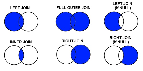
Credit: datacourses.com
- Inner join: Keep only rows that match in both datasets
- Left join: Keep all rows from the left (master) dataset
- Right join: Keep all rows from the right (using) dataset
- Full outer join: Keep all rows from both datasets
Merge Types by Relationship
Know Your Merge Type
- 1:1 — Each row matches exactly one row (person → demographics)
- m:1 — Many rows match one (students → school characteristics)
- 1:m — One row matches many (firm → firm-year panel)
- m:m — Almost always wrong! If you think you need this, reshape first.
Stata validates the relationship. When you write merge m:1, Stata checks that the using dataset actually has unique keys. If it doesn't, Stata throws an error. This is a safety feature.
R and Python do not validate. In R, merge(x, y, by = "id") performs whatever join the data produces—it doesn't verify whether it's 1:1 or m:1. The all.x, all.y, and all arguments only control which unmatched rows to keep (left, right, or outer join)—they say nothing about the merge type:
| Type | Stata | R | When to Use |
|---|---|---|---|
| 1:1 | merge 1:1 | merge(...) | Each row matches exactly one row |
| m:1 | merge m:1 | merge(..., all.x = TRUE) | Many rows match one (e.g., people → states) |
| 1:m | merge 1:m | merge(..., all.y = TRUE) | One row matches many |
In R, you must manually verify uniqueness (e.g., stopifnot(!duplicated(state_data$state))) before merging if you expect a 1:1 or m:1 relationship. Stata does this automatically.
When Merges Create Duplicates
Merges can increase your row count. This is sometimes expected and sometimes a bug.
Expected: m:1 or 1:m Merges
When merging individual data with aggregate data, rows should duplicate:
- 100 students + 5 schools → still 100 rows (each student gets their school's data)
- 50 states + 10 years of policy data → 500 state-year rows
Unexpected: Accidental Duplicates
If your row count increases unexpectedly, you probably have duplicate keys:
- Two "John Smith" entries in one dataset → each gets merged twice
- Forgot that some IDs appear multiple times
* BEFORE merging: Check for unexpected duplicates
duplicates report person_id      // Should say "all unique" for 1:1
duplicates report state          // OK to have duplicates for m:1

* Count rows before and after
count
local n_before = r(N)

merge m:1 state using "state_data.dta"

count
local n_after = r(N)

* If n_after > n_before in a m:1 merge, something is wrong!
di "Rows before: `n_before'"
di "Rows after: `n_after'"
if `n_after' > `n_before' {
    di as error "WARNING: Row count increased - check for duplicate keys!"
}
# BEFORE merging: Check for duplicates
individuals %>% count(person_id) %>% filter(n > 1) # Should be empty for 1:1
state_data %>% count(state) %>% filter(n > 1) # Should be empty
# Count rows before and after
n_before <- nrow(individuals)
merged <- merge(individuals, state_data, by = "state", all.x = TRUE)
n_after <- nrow(merged)
# Check if row count changed unexpectedly
if (n_after > n_before) {
warning("Row count increased! Check for duplicate keys in state_data")
# Find the problem
state_data %>% count(state) %>% filter(n > 1)
}# BEFORE merging: Check for duplicates
print(individuals.groupby("person_id").size().loc[lambda x: x > 1]) # Should be empty
print(state_data.groupby("state").size().loc[lambda x: x > 1]) # Should be empty
# Count rows before and after
n_before = len(individuals)
merged = individuals.merge(state_data, on="state", how="left")
n_after = len(merged)
# Check if row count changed unexpectedly
if n_after > n_before:
print("WARNING: Row count increased! Check for duplicate keys")
print(state_data.groupby("state").size().loc[lambda x: x > 1])The Row Count Rule
- 1:1 merge: Row count should stay exactly the same (or decrease if using inner join)
- m:1 merge: Row count should stay the same as master dataset
- 1:m merge: Row count will increase (one master row → many using rows)
- If row count increases when you didn't expect it, you have duplicate keys somewhere
Example: Merging Individual Data with State Data
Suppose you have individual-level data and want to add state characteristics:
person_id  state    income
1          MA       50000
2          MA       60000
3          CA       70000
4          NY       55000
state    min_wage  population
MA       15.00    7000000
CA       15.50    39500000
TX       7.25     29500000
* Load master data
use "individuals.dta", clear

* Merge: many individuals per state → m:1
merge m:1 state using "state_data.dta"

* ALWAYS check the results
tab _merge

/*
   _merge |      Freq.
----------+------------
        1 |          1    ← Only in master (NY - no state data)
        2 |          1    ← Only in using (TX - no individuals)
        3 |          3    ← Matched (MA, CA)
*/

* Investigate unmatched
list if _merge == 1   // NY had no state data
list if _merge == 2   // TX had no individuals

* Keep matched only (after understanding why others didn't match)
keep if _merge == 3
drop _merge
pacman::p_load(dplyr, haven)
individuals <- read_dta("individuals.dta")
state_data <- read_dta("state_data.dta")
# Left merge: keep all individuals, add state data where available
merged <- merge(individuals, state_data, by = "state", all.x = TRUE)
# Check for unmatched
merged %>% filter(is.na(min_wage)) # NY had no state data
# Inner merge: keep only matched
merged <- merge(individuals, state_data, by = "state")individuals = pd.read_stata("individuals.dta")
state_data = pd.read_stata("state_data.dta")
# Left join: keep all individuals, add state data where available
merged = individuals.merge(state_data, on="state", how="left", indicator=True)
# Check merge results
print(merged["_merge"].value_counts())
# Check for unmatched
print(merged[merged["min_wage"].isna()]) # NY had no state data
# Inner join: keep only matched
merged = individuals.merge(state_data, on="state", how="inner")After running tab _merge, ask yourself: Why didn't these match? Common reasons:
- Typos in merge keys ("NY" vs "New York")
- Different time periods (state data goes 2000–2010, individual data goes 1995–2015)
- Data errors or missing values in the key variable
Investigate with list state if _merge == 1 before deciding whether to keep if _merge == 3. Always document why you dropped unmatched observations.
Pre-Merge Data Cleaning
Merge variables must be exactly identical in both datasets—same name, same values, same type. Most merge problems come from subtle differences that require string cleaning.
* Check if your variable is actually numeric or string
browse, nolabel   // Shows actual values, not labels

* Common string cleaning operations:

* 1. Remove periods: "D.C." → "DC"
replace state = subinstr(state, ".", "", .)

* 2. Remove leading/trailing spaces: " MA " → "MA"
replace state = trim(state)

* 3. Extract substring: "Washington DC" → "DC"
replace state = substr(state, -2, 2)  // Last 2 characters

* 4. Convert case: "ma" → "MA"
replace state = upper(state)

* 5. Rename to match other dataset
rename statefip state

* 6. Convert string to numeric (or vice versa)
destring state_code, replace
tostring state_fips, replace
pacman::p_load(stringr)
# Common string cleaning operations:
# 1. Remove periods
data$state <- str_replace_all(data$state, "\\.", "")
# 2. Remove leading/trailing spaces
data$state <- str_trim(data$state)
# 3. Extract substring
data$state <- str_sub(data$state, -2, -1) # Last 2 characters
# 4. Convert case
data$state <- str_to_upper(data$state)
# 5. Rename to match other dataset
data <- data %>% rename(state = statefip)
# 6. Convert types
data$state_code <- as.numeric(data$state_code)
data$state_fips <- as.character(data$state_fips)# Common string cleaning operations:
# 1. Remove periods
data["state"] = data["state"].str.replace(".", "", regex=False)
# 2. Remove leading/trailing spaces
data["state"] = data["state"].str.strip()
# 3. Extract substring
data["state"] = data["state"].str[-2:] # Last 2 characters
# 4. Convert case
data["state"] = data["state"].str.upper()
# 5. Rename to match other dataset
data = data.rename(columns={"statefip": "state"})
# 6. Convert types
data["state_code"] = pd.to_numeric(data["state_code"])
data["state_fips"] = data["state_fips"].astype(str)Labels Can Be Deceiving
In Stata, when you see "Washington" in the data browser, it might actually be stored as the number 53 with a label attached. Use browse, nolabel or tab var, nolabel to see the true values. Merges use the actual values, not the labels!
Common Merge Problems
Watch Out For
- Duplicates on key: If your key isn't unique when it should be, you'll get unexpected results. Always run
duplicates reportfirst. - Case sensitivity: "MA" ≠ "ma" in Stata. Use
upper()orlower()to standardize. - Trailing spaces: "MA " ≠ "MA". Use
trim()to remove. - Different variable types: String "1" ≠ numeric 1. Convert with
destringortostring. - Labels hiding values: What looks like "California" might be stored as 6. Check with
nolabel.
Appending (Stacking) Datasets
Use append to stack datasets vertically (same variables, different observations):
* Append multiple years of data
use "data_2020.dta", clear
append using "data_2021.dta"
append using "data_2022.dta"
# Bind rows from multiple dataframes
data_all <- bind_rows(
read_dta("data_2020.dta"),
read_dta("data_2021.dta"),
read_dta("data_2022.dta")
)# Concatenate multiple dataframes
data_all = pd.concat([
pd.read_stata("data_2020.dta"),
pd.read_stata("data_2021.dta"),
pd.read_stata("data_2022.dta")
], ignore_index=True)Critical Stata Bugs That Will Break Your Analysis
Stata has some behaviors that can silently corrupt your analysis.
Missing Values Are Infinity
In Stata, missing values (.) are treated as larger than any number. This means comparisons like if x > 100 will include missing values.
* This INCLUDES missing values (dangerous!)
gen high_income = (income > 100000)

* This is what you actually want
gen high_income = (income > 100000) if !missing(income)

* Or equivalently
gen high_income = (income > 100000 & income < .)

* The ordering is: all numbers < . < .a < .b < ... < .z
* So . > 999999999 evaluates to TRUE
# R handles this more intuitively - NA propagates
high_income <- income > 100000
# Returns NA where income is NA, not TRUE
# But still be explicit about NA handling
high_income <- income > 100000 & !is.na(income)# Python/pandas handles this intuitively - NaN propagates
high_income = data["income"] > 100000
# Returns NaN where income is NaN, not True
# But still be explicit about NA handling
high_income = (data["income"] > 100000) & data["income"].notna()>, >=, or !=. Your sample sizes will be wrong, and your estimates will be biased.
egen group Silently Top-Codes
When you use egen group() to create a numeric ID from string or categorical variables, Stata uses an int by default. If you have more unique values than an int can hold (~32,000), it silently repeats the maximum value.
* DANGEROUS: If you have >32,767 unique beneficiaries,
* later IDs will all be assigned the same number!
egen bene_id = group(beneficiary_name)

* SAFE: Explicitly use a long integer
egen long bene_id = group(beneficiary_name)

* Or for very large datasets (>2 billion unique values)
egen double bene_id = group(beneficiary_name)

* Always verify you got the right number of groups
distinct beneficiary_name
assert r(ndistinct) == r(N)  // This will fail if top-coded
# R doesn't have this problem - factors work fine
data$bene_id <- as.numeric(factor(data$beneficiary_name))
# Or use dplyr
data <- data %>%
mutate(bene_id = as.numeric(factor(beneficiary_name)))# Python doesn't have this problem - uses 64-bit integers by default
data["bene_id"] = pd.factorize(data["beneficiary_name"])[0] + 1
# Verify
assert data["bene_id"].nunique() == data["beneficiary_name"].nunique()Numeric Precision
Stata's float type only has ~7 digits of precision. Large IDs stored as floats will be silently corrupted.
* float has ~7 digits of precision
* This can cause merge failures on IDs!
gen float id = 1234567890
* id is now 1234567936 (corrupted!)

* Always use long or double for IDs
gen long id = 1234567890      // integers up to ~2 billion
gen double id = 1234567890    // integers up to ~9 quadrillion

* Check if a variable might have precision issues
summarize id
* If max is > 16777216 and storage type is float, you have a problem

* Fix: compress optimizes storage types automatically
compress
# R uses double precision by default, so this is less of an issue
# But be careful with very large integers
id <- 1234567890 # Fine in R
# For extremely large integers, use bit64 package
pacman::p_load(bit64)
big_id <- as.integer64("9223372036854775807")# Python uses 64-bit integers by default, so this is less of an issue
id = 1234567890 # Fine in Python
# pandas also handles large integers well
data["id"] = pd.to_numeric(data["id"], downcast=None) # Keep full precision
# Check dtypes
print(data.dtypes)Sorting Instability
Stata's sort command is unstable—when there are ties, the order of tied observations is random and can change between runs. This causes reproducibility issues.
* DANGEROUS: Order of tied observations is random
sort state
gen observation_number = _n  // Different every time you run!

* SAFE: Break ties with a unique identifier
sort state id
gen observation_number = _n  // Now reproducible

* ALTERNATIVE: Use stable sort (preserves existing order for ties)
sort state, stable

* Best practice: Always sort by enough variables to eliminate ties
* or use stable when you don't care about tie-breaking
# R's order() is stable by default (preserves original order for ties)
data <- data[order(data$state), ]
# To be explicit about tie-breaking:
data <- data[order(data$state, data$id), ]
# dplyr::arrange() is also stable
pacman::p_load(dplyr)
data <- data %>% arrange(state, id)# pandas sort_values() has kind='stable' option
data = data.sort_values('state', kind='stable')
# Better: explicitly break ties
data = data.sort_values(['state', 'id'])
# Note: default sort is 'quicksort' which is unstable_n for observation numbers or by: gen first = _n == 1), your results will differ across runs, making your analysis non-reproducible.
Variable Abbreviation
By default, Stata allows you to abbreviate variable names. This is dangerous—your code can silently operate on the wrong variable if you add new variables later.
* Suppose you have: income, age, education
summarize inc  // Works! Stata abbreviates to "income"

* Later, you add: income_spouse
summarize inc  // ERROR: "inc" is ambiguous (income vs income_spouse)
* Or worse: no error, wrong variable used silently

* SOLUTION: Disable variable abbreviation at the start of every do-file
set varabbrev off

* Now Stata requires exact variable names
summarize income  // Must use full name
# R does NOT allow variable abbreviation by default
# You must use exact column names
summary(data$income) # Must be exact
# Partial matching only happens with $ on lists, not data frames
# This is generally not a problem in R# Python does NOT allow column abbreviation
# You must use exact column names
data['income'].describe() # Must be exact
# Autocomplete in IDEs helps with long names
# No risk of silent abbreviation errorsset varabbrev off at the top of every do-file.
Defensive Coding Habits
- Put
set varabbrev offat the top of every do-file - Always use
if !missing(x)with inequality comparisons - Always use
egen longoregen doublefor group IDs - Sort by enough variables to eliminate ties, or use
sort ..., stable - Run
compressafter loading data to optimize storage types - Use
assertliberally to catch problems early
Practice Exercise
Test your understanding with this data wrangling challenge.
Scenario
You have two datasets:
- students.csv: One row per student with columns
student_id,school_id,test_score - schools.csv: One row per school with columns
school_id,school_type(public/private),total_enrollment
Task: Create a dataset where each row is a student, with their school's characteristics added.
Questions to answer before coding:
- What type of merge is this? (1:1, m:1, 1:m, m:m)
- After the merge, how many rows should you have?
- What should you check before merging?
Click to see answers + code
Answers:
- m:1 — Many students per school, one school record per school
- Same number of rows as students.csv (school info gets duplicated to each student)
- Check that
school_idis unique in schools.csv:duplicates report school_id
* Stata solution
import delimited "students.csv", clear
count  // Note: N students

merge m:1 school_id using "schools.dta"
tab _merge  // All should match (or investigate non-matches)

count  // Should equal original N students
keep if _merge == 3
drop _mergeFound something unclear or have a suggestion? Email [email protected].