A Complete Research Project
Walking through a project like a student figuring it out
This worked example follows the thought process of a student working through an empirical research project. Instead of presenting polished steps, we'll show the reasoning behind each decision—the "why am I doing this?" that often gets lost in tutorials.
We're replicating part of French & Gumus (2024), "Hit-and-Run or Hit-and-Stay? Unintended Effects of a Stricter BAC Limit." But more importantly, we're showing how you'd approach a project like this from scratch.
What You'll Learn
- How to think through a research question and check if it's feasible
- How to figure out what data you need (and where to get it)
- How to decide on a unit of analysis and why it matters
- How to deal with datasets that don't line up
- The thought process behind merging, aggregating, and cleaning
- How to actually run a diff-in-diff and interpret it
The Research Project Pipeline
Most empirical projects follow roughly the same flow:
This tutorial walks through each step using a real research question. We'll show not just what to do, but why — the reasoning that guides each decision.
1. Starting a Research Project
So you want to do an empirical research project. You need three things:
Here's an idea that has all three:
The Question
Do stricter drunk driving laws reduce hit-and-run crashes?
Between 1983 and 2004, all 50 U.S. states lowered their legal blood alcohol content (BAC) limit from 0.10 to 0.08. The policy goal was to reduce drunk driving fatalities. But did it have unintended effects? Specifically: might stricter penalties cause drunk drivers who cause crashes to flee the scene to avoid arrest?
The Data
- Outcome: Fatal hit-and-run crashes (from FARS—the national crash database)
- Treatment: When each state adopted the 0.08 BAC law (from APIS)
- Controls: Unemployment, income, and other policies (from FRED and other sources)
The Identification Strategy
We use a difference-in-differences design. States adopted 0.08 BAC laws at different times, so we compare changes in hit-and-run crashes in states that just adopted the law versus states that haven't adopted yet.
Sample adoption dates:
| State | Adopted |
|---|---|
| Utah | 1983 |
| Oregon | 1983 |
| California | 1990 |
| Texas | 1999 |
| Minnesota | 2005 |
The identifying assumption:
In the absence of the 0.08 law, hit-and-run fatalities would have followed parallel trends across early-adopting and late-adopting states.
We test this by checking that pre-treatment trends are similar (the "event study" plot).
Checkpoint: Do We Have All Three?
- Question: Does the 0.08 BAC law affect hit-and-run crashes? ✓
- Data: State-year panel of crashes, policies, and controls. ✓
- Identification: DiD exploiting staggered adoption with parallel trends test. ✓
We're ready to start building our dataset.
2. Setting Up Your Project
Before we start coding, let's set up a proper folder structure. This follows the standard economics project layout discussed in the Project Organization tutorial.
Folder Structure
bac_replication/
├── master.do              # (or master.R, main.py) Runs everything
├── README.md
│
├── build/
│   ├── input/             # Raw data (NEVER modify!)
│   │   ├── fars/          # FARS crash data by year
│   │   ├── apis/          # BAC law adoption dates
│   │   └── fred/          # Economic controls
│   ├── code/
│   │   ├── 01_download_fars.do
│   │   ├── 02_import_bac_dates.do
│   │   ├── 03_aggregate_crashes.do
│   │   └── 04_merge_all.do
│   └── output/
│       └── analysis_data.dta
│
├── analysis/
│   ├── code/
│   │   ├── 01_summary_stats.do
│   │   ├── 02_twfe_regression.do
│   │   └── 03_event_study.do
│   └── output/
│       ├── tables/
│       └── figures/
│
└── paper/
The Master Script
Create a master script that runs everything with one click. This is critical for reproducibility.
/*==============================================================================
    Master Do-File: BAC Laws and Hit-and-Run Crashes
    Replication of French & Gumus (2024)
==============================================================================*/

clear all
set more off

* ============ CHANGE THIS PATH ============
global root "/Users/yourname/Dropbox/bac_replication"
* ==========================================

* Define paths
global build    "$root/build"
global analysis "$root/analysis"

* Build data
do "$build/code/01_download_fars.do"
do "$build/code/02_import_bac_dates.do"
do "$build/code/03_aggregate_crashes.do"
do "$build/code/04_merge_all.do"

* Run analysis
do "$analysis/code/01_summary_stats.do"
do "$analysis/code/02_twfe_regression.do"
do "$analysis/code/03_event_study.do"

di "Done! Results in $analysis/output/"
#==============================================================================
# Master Script: BAC Laws and Hit-and-Run Crashes
# Replication of French & Gumus (2024)
#==============================================================================
rm(list = ls())
# ============ CHANGE THIS PATH ============
root <- "/Users/yourname/Dropbox/bac_replication"
# ==========================================
# Define paths
build <- file.path(root, "build")
analysis <- file.path(root, "analysis")
# Build data
source(file.path(build, "code", "01_download_fars.R"))
source(file.path(build, "code", "02_import_bac_dates.R"))
source(file.path(build, "code", "03_aggregate_crashes.R"))
source(file.path(build, "code", "04_merge_all.R"))
# Run analysis
source(file.path(analysis, "code", "01_summary_stats.R"))
source(file.path(analysis, "code", "02_twfe_regression.R"))
source(file.path(analysis, "code", "03_event_study.R"))
cat("Done! Results in", file.path(analysis, "output"))#==============================================================================
# Master Script: BAC Laws and Hit-and-Run Crashes
# Replication of French & Gumus (2024)
#==============================================================================
import os
from pathlib import Path
# ============ CHANGE THIS PATH ============
ROOT = Path("/Users/yourname/Dropbox/bac_replication")
# ==========================================
# Define paths
BUILD = ROOT / "build"
ANALYSIS = ROOT / "analysis"
# Build data
exec(open(BUILD / "code" / "01_download_fars.py").read())
exec(open(BUILD / "code" / "02_import_bac_dates.py").read())
exec(open(BUILD / "code" / "03_aggregate_crashes.py").read())
exec(open(BUILD / "code" / "04_merge_all.py").read())
# Run analysis
exec(open(ANALYSIS / "code" / "01_summary_stats.py").read())
exec(open(ANALYSIS / "code" / "02_twfe_regression.py").read())
exec(open(ANALYSIS / "code" / "03_event_study.py").read())
print(f"Done! Results in {ANALYSIS / 'output'}")Understanding the Data Workflow
Before we dive into data sources, let's understand the overall strategy for building an analysis dataset. This is the core skill of empirical research.
The Multi-Source Data Workflow
In most empirical projects, your final dataset comes from multiple sources that need to be combined. The workflow is:
- Identify your data sources — What datasets contain the variables you need?
- Clean each dataset separately — Fix coding issues, handle missing values, rename variables consistently
- Aggregate to a common unit — Each dataset might start at different levels (crash-level, county-level, etc.), but they all need to end up at the same unit of analysis (state-year in our case)
- Standardize identifiers — All datasets need the same ID variables (e.g., state FIPS codes) so they can be linked
- Merge everything together — Combine all cleaned datasets into one analysis file
- Run all analyses on the merged dataset — Your regressions, summary stats, and figures all use this single file
Why Separate Cleaning Steps?
Each data source has its own quirks: different variable names, different coding schemes, different time periods, different geographic units. If you try to merge raw data directly, you'll create a mess. By cleaning each source into a uniform format first, the merge step becomes trivial — just a simple join on state + year.
In our project, we'll have:
- FARS → crash-level data → collapse to state-year counts
- APIS → state-level policy dates → expand to state-year panel via merge
- FRED/BLS → economic data → already at state-year level
Each gets cleaned in its own script, standardized to state FIPS + year, then merged in a final step. Let's see how this works.
3. Finding Your Data Sources
Now comes the hard part: what data do we actually need? Let's think through this systematically. For a diff-in-diff, we need:
- An outcome variable (Y) — what we're measuring (hit-and-run crashes)
- A treatment variable (D) — when/where the policy was in effect
- Controls (X) — other factors that might affect the outcome
So where do we find each of these? This is where you start Googling.
The Outcome: Where Do We Get Hit-and-Run Data?
We need data on fatal hit-and-run crashes. After some searching, we find the Fatality Analysis Reporting System (FARS) — a census of every fatal traffic crash in the United States maintained by NHTSA. Each row is a crash.
- Source: NHTSA (National Highway Traffic Safety Administration)
- URL: nhtsa.gov/research-data/fatality-analysis-reporting-system-fars
- Unit: One row per crash (crash-level data)
- Key variable:
HIT_RUNin the Vehicle file
Wait — how did we know this data existed? Honestly, a lot of research starts with asking: "What datasets exist that measure what I care about?" For traffic crashes, FARS is the gold standard. If you're studying something else, you might need to dig around on government websites, data repositories like ICPSR, or look at what data other papers in your area use.
HIT_RUN coding (varies by year):
- Pre-2005: 0=No, 1=Yes, 2=Unknown, 3=Not Reported
- 2005+: 0=No, 1-4=Yes (various categories)
Note: You'll often discover these coding details only after downloading the data and reading the documentation. That's normal.
The Treatment: When Did Each State Adopt the 0.08 Law?
For our diff-in-diff, we need to know exactly when each state adopted the 0.08 BAC limit. This is our treatment variable. After searching, we find the Alcohol Policy Information System (APIS) from NIAAA, which tracks alcohol-related laws by state.
- Source: NIAAA
- URL: alcoholpolicy.niaaa.nih.gov
- Unit: One row per state
- Key variable: 0.08 BAC adoption date
Why APIS and not somewhere else? APIS is authoritative because NIAAA (the National Institute on Alcohol Abuse and Alcoholism) specifically compiles policy adoption dates. You could also find this information by reading the actual state statutes, but APIS has done that work for you.
Controls: What Else Might Affect Hit-and-Runs?
This is where you have to think carefully. What factors other than BAC laws might affect hit-and-run rates, and might also be correlated with when states adopt BAC laws?
Fixed effects control for time-invariant state characteristics and common year shocks. But they don't control for things that vary both across states and over time. If recessions hit some states harder than others, and those same states happen to adopt BAC laws at different times, we could have a problem.
Economic conditions are an obvious candidate — unemployment affects driving behavior and crash rates. We can get this from FRED (Federal Reserve Economic Data):
- Source: FRED (Federal Reserve Economic Data)
- Unit: One row per state-year
- Variables: Unemployment rate, per capita income
* 01_download_fars.do - Download FARS data
* Run from: $build/code/

* Download FARS data (example for one year)
copy "https://static.nhtsa.gov/nhtsa/downloads/FARS/2000/National/FARS2000NationalCSV.zip" ///
     "$build/input/fars/fars_2000.zip", replace

* Unzip to input folder
cd "$build/input/fars"
unzipfile "fars_2000.zip", replace

* Import and save as Stata format
import delimited "accident.csv", clear
save "$build/input/fars/accident_2000.dta", replace

import delimited "vehicle.csv", clear
save "$build/input/fars/vehicle_2000.dta", replace
# 01_download_fars.R - Download FARS data
pacman::p_load(tidyverse)
# Download FARS data
url <- "https://static.nhtsa.gov/nhtsa/downloads/FARS/2000/National/FARS2000NationalCSV.zip"
dest <- file.path(build, "input", "fars", "fars_2000.zip")
download.file(url, dest)
# Unzip
unzip(dest, exdir = file.path(build, "input", "fars", "2000"))
# Read and save
accident <- read_csv(file.path(build, "input", "fars", "2000", "accident.csv"))
write_rds(accident, file.path(build, "input", "fars", "accident_2000.rds"))# 01_download_fars.py - Download FARS data
import pandas as pd
import requests
import zipfile
from pathlib import Path
# Download FARS data
url = "https://static.nhtsa.gov/nhtsa/downloads/FARS/2000/National/FARS2000NationalCSV.zip"
dest = BUILD / "input" / "fars" / "fars_2000.zip"
dest.parent.mkdir(parents=True, exist_ok=True)
response = requests.get(url)
with open(dest, 'wb') as f:
f.write(response.content)
# Extract
with zipfile.ZipFile(dest) as z:
z.extractall(BUILD / "input" / "fars" / "2000")
# Read and save
accident = pd.read_csv(BUILD / "input" / "fars" / "2000" / "accident.csv",
encoding='latin-1')
accident.to_parquet(BUILD / "input" / "fars" / "accident_2000.parquet")4. Deciding on Your Unit of Analysis
Here's a question that trips up a lot of students: What should each row in your final dataset represent?
This isn't obvious! You have to think about what makes sense for your research design. Let's reason through it:
The question we're trying to answer:
"Did states that adopted 0.08 BAC laws see different changes in hit-and-run crashes compared to states that hadn't adopted the law yet?"
This question is fundamentally about states and how they change over time. So our unit of analysis should be state-year: one observation for each state in each year.
For our DiD, we need a state-year panel. This means:
- Each row is one state in one year
- 50 states × 27 years (1982-2008) = 1,350 potential observations
- Columns include: outcome (hit-run fatalities), treatment (BAC law), controls
The Problem: Our Data Isn't at State-Year Level
Here's where things get tricky. Our raw data comes at different levels:
| Dataset | Current Unit | Target Unit | Action |
|---|---|---|---|
| FARS crashes | Crash | State-year | Aggregate up (count crashes) |
| BAC laws | State | State-year | Expand (one row per year) |
| FRED controls | State-year | State-year | Ready to merge |
This table tells us what we need to do with each dataset. But why these specific actions?
Aggregating FARS: From Crashes to Counts
Our outcome is the number of hit-and-run crashes in each state-year. But FARS gives us individual crash records. We need to aggregate.
Think about it this way: at the crash level, there's no variation to explain. Each crash either is or isn't a hit-and-run — that's it. But we're not asking "what makes a crash more likely to be hit-and-run?" We're asking "does the BAC law affect how many hit-and-run crashes happen?" That's a count, and counts only exist when you aggregate observations.
So we need to collapse the crash-level data: count how many hit-and-run crashes happened in each state-year.
* 03_aggregate_crashes.do - Aggregate FARS to state-year
* Run from: $build/code/

* Load vehicle file (has hit-run indicator)
use "$build/input/fars/vehicle_2000.dta", clear

* Code hit-run indicator (codes 1-4 = hit-and-run)
gen hit_run = inlist(hit_run, 1, 2, 3, 4)

* Collapse to crash level (any vehicle fled = hit-run crash)
collapse (max) hit_run, by(st_case)
tempfile vehicle_hitrun
save `vehicle_hitrun'

* Merge with accident file to get state and year
use "$build/input/fars/accident_2000.dta", clear
merge 1:1 st_case using `vehicle_hitrun'

* Aggregate to state-year
collapse (count) total_crashes=st_case ///
         (sum) hr_crashes=hit_run, ///
         by(state year)

gen nhr_crashes = total_crashes - hr_crashes
save "$build/output/state_year_crashes.dta", replace
# 03_aggregate_crashes.R - Aggregate FARS to state-year
pacman::p_load(tidyverse)
# Load vehicle file and code hit-run
vehicle <- read_rds(file.path(build, "input", "fars", "vehicle_2000.rds")) %>%
mutate(hit_run = hit_run %in% c(1, 2, 3, 4))
# Collapse to crash level (any vehicle fled = hit-run crash)
crash_hitrun <- vehicle %>%
group_by(st_case) %>%
summarize(hit_run = max(hit_run))
# Merge with accident file
accident <- read_rds(file.path(build, "input", "fars", "accident_2000.rds"))
crashes <- accident %>%
left_join(crash_hitrun, by = "st_case")
# Aggregate to state-year
state_year <- crashes %>%
group_by(state, year) %>%
summarize(
total_crashes = n(),
hr_crashes = sum(hit_run, na.rm = TRUE),
nhr_crashes = total_crashes - hr_crashes,
.groups = "drop"
)
write_rds(state_year, file.path(build, "output", "state_year_crashes.rds"))# 03_aggregate_crashes.py - Aggregate FARS to state-year
import pandas as pd
# Load vehicle file and code hit-run
vehicle = pd.read_parquet(BUILD / "input" / "fars" / "vehicle_2000.parquet")
vehicle['hit_run'] = vehicle['hit_run'].isin([1, 2, 3, 4])
# Collapse to crash level
crash_hitrun = vehicle.groupby('st_case')['hit_run'].max().reset_index()
# Merge with accident file
accident = pd.read_parquet(BUILD / "input" / "fars" / "accident_2000.parquet")
crashes = accident.merge(crash_hitrun, on='st_case', how='left')
# Aggregate to state-year
state_year = crashes.groupby(['state', 'year']).agg(
total_crashes=('st_case', 'count'),
hr_crashes=('hit_run', 'sum')
).reset_index()
state_year['nhr_crashes'] = state_year['total_crashes'] - state_year['hr_crashes']
state_year.to_parquet(BUILD / "output" / "state_year_crashes.parquet")* Create complete state-year panel
* (ensures we have rows even for state-years with 0 crashes)
preserve
keep state
duplicates drop
expand 27 // 1982-2008
bysort state: gen year = 1981 + _n
tempfile panel
save `panel'
restore
* Merge crash data onto complete panel
use `panel', clear
merge 1:1 state year using "state_year_crashes.dta"
* Fill missing values with zeros (not missing!)
foreach var in total_crashes hr_crashes nhr_crashes {
replace `var' = 0 if missing(`var')
}# Create complete state-year panel
complete_panel <- expand.grid(
state = unique(crashes$state),
year = 1982:2008
)
# Merge and fill zeros
state_year <- complete_panel %>%
left_join(state_year, by = c("state", "year")) %>%
mutate(across(c(total_crashes, hr_crashes, nhr_crashes),
~replace_na(., 0)))# Create complete state-year panel
import itertools
states = crashes['state'].unique()
years = range(1982, 2009)
complete_panel = pd.DataFrame(
list(itertools.product(states, years)),
columns=['state', 'year']
)
# Merge and fill zeros
state_year = complete_panel.merge(state_year, on=['state', 'year'], how='left')
state_year = state_year.fillna({'total_crashes': 0, 'hr_crashes': 0, 'nhr_crashes': 0})5. Merging Your Datasets
At this point we have three separate datasets:
- Crash counts by state-year (from FARS)
- BAC law adoption dates by state (from APIS)
- Economic controls by state-year (from FRED)
We need to combine them into one analysis dataset. This is called merging, and it's where a lot of bugs happen. Let's think through each merge carefully.
A Quick Primer on Merge Types
Before we merge, we need to understand how different merge types work. The key question is: how many rows in dataset A match each row in dataset B?
| Merge Type | When to Use | Example |
|---|---|---|
| 1:1 | Each row in master matches exactly one row in using | Merge state-year crashes with state-year unemployment |
| m:1 (many-to-one) | Multiple master rows match one using row | Merge state-year data with state-level BAC dates (one date applies to all years) |
| 1:m (one-to-many) | One master row matches multiple using rows | Merge state data to person-level data (each state has many people) |
| m:m | Almost never! Creates Cartesian product. | Usually a mistake. Check your data. |
Step 1: Merge BAC Adoption Dates (m:1) — The "Expand" Step
BAC adoption dates are at the state level (one row per state). We're merging them to state-year data, so many state-years match one state. This is an m:1 merge.
Understanding the Expand Operation
This m:1 merge is how we expand state-level data to state-year level. Here's what happens:
- Before merge: BAC dates have 50 rows (one per state), each with a single adoption year
- After merge: Each state's adoption year appears in all 27 rows for that state (one per year, 1982-2008)
The merge effectively "copies" the state-level variable to every state-year observation. This is the opposite of collapse: collapse reduces rows (many → one), while expand via merge replicates values across rows (one → many).
* 04_merge_all.do - Merge all datasets
* Run from: $build/code/

* Load BAC adoption dates (one row per state)
import delimited "$build/input/apis/bac08_adoption_dates.csv", clear
gen adoption_year = year(date(effective_date, "YMD"))
keep state_fips adoption_year
tempfile bac_dates
save `bac_dates'

* Merge with state-year fatality data (m:1)
use "$build/output/state_year_crashes.dta", clear
merge m:1 state_fips using `bac_dates'

* Check merge results
tab _merge
* All should be matched (_merge == 3)
drop _merge

* Create treatment variables
gen event_time = year - adoption_year
gen treated = (event_time >= 0)
# 04_merge_all.R - Merge all datasets
# Load BAC adoption dates
bac_dates <- read_csv(file.path(build, "input", "apis", "bac08_adoption_dates.csv")) %>%
mutate(
effective_date = as.Date(effective_date),
adoption_year = year(effective_date)
) %>%
select(state_fips, adoption_year)
# Load crash data
state_year <- read_rds(file.path(build, "output", "state_year_crashes.rds"))
# Merge with state-year data
state_year <- state_year %>%
left_join(bac_dates, by = "state_fips") %>%
mutate(
event_time = year - adoption_year,
treated = as.integer(event_time >= 0)
)
# Verify no missing adoption years
stopifnot(sum(is.na(state_year$adoption_year)) == 0)# 04_merge_all.py - Merge all datasets
import pandas as pd
# Load BAC adoption dates
bac_dates = pd.read_csv(BUILD / "input" / "apis" / "bac08_adoption_dates.csv")
bac_dates['effective_date'] = pd.to_datetime(bac_dates['effective_date'])
bac_dates['adoption_year'] = bac_dates['effective_date'].dt.year
# Load crash data
state_year = pd.read_parquet(BUILD / "output" / "state_year_crashes.parquet")
# Merge with state-year data
state_year = state_year.merge(
bac_dates[['state_fips', 'adoption_year']],
on='state_fips',
how='left'
)
# Create treatment variables
state_year['event_time'] = state_year['year'] - state_year['adoption_year']
state_year['treated'] = (state_year['event_time'] >= 0).astype(int)
# Verify no missing
assert state_year['adoption_year'].notna().all()Step 2: Merge Economic Controls (1:1)
FRED data is already at the state-year level, matching our analysis data. This is a 1:1 merge.
* Merge unemployment (1:1 on state-year)
merge 1:1 state_fips year using "$build/input/fred/unemployment.dta", nogen

* Merge income (1:1 on state-year)
merge 1:1 state_fips year using "$build/input/fred/income.dta", nogen

* Create outcome variables
gen ln_hr = ln(hr_crashes + 1)
gen ln_nhr = ln(nhr_crashes + 1)

* Save final analysis dataset
save "$build/output/analysis_data.dta", replace
# Load controls
unemployment <- read_rds(file.path(build, "input", "fred", "unemployment.rds"))
income <- read_rds(file.path(build, "input", "fred", "income.rds"))
# Merge controls
state_year <- state_year %>%
left_join(unemployment, by = c("state_fips", "year")) %>%
left_join(income, by = c("state_fips", "year")) %>%
mutate(
ln_hr = log(hr_crashes + 1),
ln_nhr = log(nhr_crashes + 1)
)
# Save final analysis dataset
write_rds(state_year, file.path(build, "output", "analysis_data.rds"))# Load and merge controls
unemployment = pd.read_parquet(BUILD / "input" / "fred" / "unemployment.parquet")
income = pd.read_parquet(BUILD / "input" / "fred" / "income.parquet")
state_year = state_year.merge(unemployment, on=['state_fips', 'year'], how='left')
state_year = state_year.merge(income, on=['state_fips', 'year'], how='left')
# Create outcome variables
import numpy as np
state_year['ln_hr'] = np.log(state_year['hr_crashes'] + 1)
state_year['ln_nhr'] = np.log(state_year['nhr_crashes'] + 1)
# Save final analysis dataset
state_year.to_parquet(BUILD / "output" / "analysis_data.parquet")Final Analysis Dataset
- Unit: State-year (50 states × 27 years = 1,350 obs)
- Outcome:
ln_hr(log hit-run fatalities + 1) - Treatment:
treated(1 if 0.08 BAC law in effect) - Event time:
event_time(years since/until adoption) - Controls: unemployment, income
- Fixed effects: State and year
6. Descriptive Statistics
At this point, many students want to jump straight to the regression. Don't. You should always look at your data first. Here's why:
- Did the merge work? (Do you have the right number of observations?)
- Are there weird values that suggest coding errors?
- Do treated and control groups look reasonably similar on observables?
- Is there enough variation to detect an effect?
Create summary statistics showing how treated and untreated observations compare.
Quick Review: Variable Types
Continuous Variables
Variables that can take any value in a range (income, crashes, unemployment rate). Report mean (SD).
Categorical Variables
Variables that take discrete categories (region, treatment group, policy type). Report counts and percentages.
Summary Statistics Table
Create a table showing Total, Treated (post-treatment obs), and Untreated (pre-treatment obs):
* 01_summary_stats.do - Descriptive statistics
* Run from: $analysis/code/

use "$build/output/analysis_data.dta", clear

* Overall summary
summarize hr_crashes nhr_crashes unemployment income

* By treatment status
bysort treated: summarize hr_crashes nhr_crashes

* More detailed: mean and SD
tabstat hr_crashes nhr_crashes unemployment, ///
    by(treated) stats(mean sd n) columns(statistics)

* Publication table with estout
estpost tabstat hr_crashes nhr_crashes unemployment income, ///
    by(treated) stats(mean sd) columns(statistics)
esttab using "$analysis/output/tables/summary_stats.tex", ///
    cells("mean(fmt(2)) sd(fmt(2))") replace
# 01_summary_stats.R - Descriptive statistics
pacman::p_load(tidyverse, kableExtra)
# Load analysis data
state_year <- read_rds(file.path(build, "output", "analysis_data.rds"))
# Summary by treatment status
summary_table <- state_year %>%
group_by(treated) %>%
summarize(
across(c(hr_crashes, nhr_crashes, unemployment, income),
list(mean = ~mean(., na.rm = TRUE),
sd = ~sd(., na.rm = TRUE))),
n = n()
)
# Overall summary
overall <- state_year %>%
summarize(
across(c(hr_crashes, nhr_crashes, unemployment, income),
list(mean = mean, sd = sd)),
n = n()
) %>%
mutate(treated = "Total")
# Combine and save
summary_all <- bind_rows(summary_table, overall)
write_csv(summary_all, file.path(analysis, "output", "tables", "summary_stats.csv"))# 01_summary_stats.py - Descriptive statistics
import pandas as pd
# Load analysis data
state_year = pd.read_parquet(BUILD / "output" / "analysis_data.parquet")
# Summary by treatment status
summary_by_treated = state_year.groupby('treated')[
['hr_crashes', 'nhr_crashes', 'unemployment', 'income']
].agg(['mean', 'std', 'count'])
# Overall summary
overall = state_year[
['hr_crashes', 'nhr_crashes', 'unemployment', 'income']
].agg(['mean', 'std', 'count'])
print("By Treatment Status:")
print(summary_by_treated)
print("\nOverall:")
print(overall)
# Save
summary_by_treated.to_csv(ANALYSIS / "output" / "tables" / "summary_stats.csv")Your summary statistics table should look something like:
| Variable | Total | Untreated | Treated |
|---|---|---|---|
| Hit-run crashes | 45.2 (67.3) | 38.4 (58.2) | 52.1 (74.8) |
| Non-hit-run crashes | 812 (892) | 856 (934) | 768 (847) |
| Unemployment (%) | 5.6 (1.8) | 5.8 (1.9) | 5.4 (1.7) |
| N (state-years) | 1,350 | 675 | 675 |
Notes: Standard deviations in parentheses. Untreated = pre-0.08 BAC law; Treated = post-0.08 BAC law.
7. Running the Diff-in-Diff
Now we're finally ready to estimate our treatment effect. But what regression should we run?
The basic idea of diff-in-diff is simple: compare the change in outcomes for treated units to the change in outcomes for control units. With staggered adoption (where different states adopt at different times), we use two-way fixed effects (TWFE): state fixed effects absorb time-invariant state characteristics, and year fixed effects absorb common shocks that hit all states.
The Simple Specification
The simplest specification estimates a single average treatment effect:
* 02_twfe_regression.do - TWFE DiD regression
* Run from: $analysis/code/

* Install reghdfe if needed
* ssc install reghdfe
* ssc install ftools

use "$build/output/analysis_data.dta", clear

* Simple TWFE DiD
reghdfe ln_hr treated unemployment, ///
    absorb(state_fips year) cluster(state_fips)

* Interpretation: coefficient on 'treated' is the DiD estimate
* Positive = hit-run crashes increased after 0.08 law
# 02_twfe_regression.R - TWFE DiD regression
pacman::p_load(fixest, tidyverse)
# Load analysis data
state_year <- read_rds(file.path(build, "output", "analysis_data.rds"))
# Simple TWFE DiD
did_model <- feols(
ln_hr ~ treated + unemployment | state_fips + year,
data = state_year,
cluster = ~state_fips
)
summary(did_model)# 02_twfe_regression.py - TWFE DiD regression
import pandas as pd
import pyfixest as pf
# Load analysis data
state_year = pd.read_parquet(BUILD / "output" / "analysis_data.parquet")
# Simple TWFE DiD
results = pf.feols(
'ln_hr ~ treated + unemployment | state_fips + year',
data=state_year, vcov={'CRV1': 'state_fips'}
)
results.summary()Event Study: Testing the Identifying Assumption
The simple regression gives us an answer, but should we believe it? Diff-in-diff only works if the parallel trends assumption holds: treated and control states would have followed similar paths absent treatment.
We can't directly test this (we never observe the counterfactual), but we can do the next best thing: check whether pre-treatment trends were parallel. If they were, that's suggestive evidence that post-treatment trends would have been parallel too.
This is what an event study does. Instead of estimating one treatment effect, we estimate separate effects for each period relative to treatment:
* 03_event_study.do - Event study
* Run from: $analysis/code/

use "$build/output/analysis_data.dta", clear

* Create event time dummies (bin endpoints at -5 and +10)
gen event_time_binned = event_time
replace event_time_binned = -5 if event_time < -5
replace event_time_binned = 10 if event_time > 10

* Create dummies (omit -1 as reference)
tab event_time_binned, gen(et_)

* Event study regression
reghdfe ln_hr et_* unemployment, ///
    absorb(state_fips year) cluster(state_fips)

* Plot coefficients
coefplot, vertical keep(et_*) ///
    yline(0) xline(5.5, lpattern(dash)) ///
    title("Event Study: Hit-and-Run Crashes") ///
    xtitle("Years Since 0.08 BAC Law") ytitle("Coefficient")

graph export "$analysis/output/figures/event_study.png", replace width(1200)
# 03_event_study.R - Event study
pacman::p_load(fixest, tidyverse)
# Load analysis data
state_year <- read_rds(file.path(build, "output", "analysis_data.rds"))
# IMPORTANT: Handle never-treated units properly
# Never-treated states don't have a meaningful "time to treatment"
# Set them to a value outside the data range (e.g., -1000)
# Then exclude with ref = c(-1, -1000)
#
# Note: In this BAC dataset, ALL states eventually adopted (no never-treated),
# but we show the general pattern that works for any dataset.
state_year <- state_year %>%
mutate(
# If there were never-treated states, they'd have NA for adoption_year
# Set their event_time to -1000 (outside data range)
event_time = ifelse(is.na(adoption_year), -1000, year - adoption_year),
# Binary: ever treated vs never treated
ever_treated = !is.na(adoption_year)
)
# Bin endpoints to avoid sparse cells at extremes
state_year <- state_year %>%
mutate(event_time_binned = case_when(
event_time == -1000 ~ -1000, # Keep never-treated separate
event_time <= -5 ~ -5, # Bin early periods
event_time >= 10 ~ 10, # Bin late periods
TRUE ~ event_time
))
# Event study with fixest
# i(event_time_binned, ever_treated, ref = c(-1, -1000)) means:
# - Create dummies for each event_time_binned value
# - Interact with ever_treated indicator
# - Exclude t=-1 (reference period) AND t=-1000 (never-treated)
es_model <- feols(
ln_hr ~ i(event_time_binned, ever_treated, ref = c(-1, -1000)) + unemployment | state_fips + year,
data = state_year,
cluster = ~state_fips
)
# Plot (fixest has built-in event study plotting)
png(file.path(analysis, "output", "figures", "event_study.png"), width = 1200, height = 800)
iplot(es_model,
main = "Event Study: Hit-and-Run Crashes",
xlab = "Years Since 0.08 BAC Law",
ylab = "Coefficient")
dev.off()# 03_event_study.py - Event study
import pandas as pd
import matplotlib.pyplot as plt
# Load analysis data
state_year = pd.read_parquet(BUILD / "output" / "analysis_data.parquet")
# Create event time dummies
df = state_year.copy()
df['event_time_binned'] = df['event_time'].clip(-5, 10)
# Create dummies (excluding -1 as reference)
event_times = sorted([et for et in df['event_time_binned'].unique() if et != -1])
for et in event_times:
col_name = f'et_{et}' if et >= 0 else f'et_m{abs(et)}'
df[col_name] = (df['event_time_binned'] == et).astype(int)
# Run regression with all event time dummies
# Then extract coefficients and plot with matplotlib
# (see full code in repository)
# Save figure
plt.savefig(ANALYSIS / "output" / "figures" / "event_study.png", dpi=300)Interpreting the Event Study
- Pre-trends (t < 0): Coefficients should be close to zero and statistically insignificant. This supports the parallel trends assumption.
- t = -1: This is the reference period (normalized to zero).
- Post-treatment (t ≥ 0): These show the dynamic treatment effect.
8. Publication-Ready Output
The final step in empirical research is presenting your results clearly. Publication-ready output means tables and figures that are:
- Self-contained: A reader should understand the figure without reading the full paper
- Precisely formatted: Consistent decimal places, clear labels, appropriate significance stars
- Reproducible: Generated by code, not manually edited in Excel
Creating Publication Tables
Regression tables need to convey a lot of information compactly. A good table includes:
- Coefficient estimates with appropriate decimal precision (usually 3 digits)
- Standard errors in parentheses below coefficients
- Significance stars following a stated convention (*, **, ***)
- Sample size and fit statistics (N, R²) at the bottom
- Clear column headers identifying each specification
We export to LaTeX format because it integrates seamlessly with academic papers and maintains precise formatting. The code below creates a table comparing hit-and-run vs. non-hit-and-run crashes:
* 04_tables.do - Publication tables
* Run from: $analysis/code/

use "$build/output/analysis_data.dta", clear

* Run both specifications
reghdfe ln_hr treated unemployment, absorb(state_fips year) cluster(state_fips)
est store hr_model

reghdfe ln_nhr treated unemployment, absorb(state_fips year) cluster(state_fips)
est store nhr_model

* Export to LaTeX
esttab hr_model nhr_model using "$analysis/output/tables/table2.tex", ///
    cells(b(star fmt(3)) se(par fmt(3))) ///
    star(* 0.10 ** 0.05 *** 0.01) ///
    stats(N r2, fmt(%9.0fc %9.3f) labels("Observations" "R-squared")) ///
    mtitles("Hit-Run" "Non-Hit-Run") ///
    title("Effect of 0.08 BAC Laws on Crashes") ///
    replace
# 04_tables.R - Publication tables
pacman::p_load(fixest, modelsummary, tidyverse)
# Load analysis data
state_year <- read_rds(file.path(build, "output", "analysis_data.rds"))
# Estimate both models
hr_model <- feols(ln_hr ~ treated + unemployment | state_fips + year,
data = state_year, cluster = ~state_fips)
nhr_model <- feols(ln_nhr ~ treated + unemployment | state_fips + year,
data = state_year, cluster = ~state_fips)
# Create publication table
modelsummary(
list("Hit-Run" = hr_model, "Non-Hit-Run" = nhr_model),
stars = c('*' = .1, '**' = .05, '***' = .01),
gof_map = c("nobs", "r.squared"),
output = file.path(analysis, "output", "tables", "table2.tex")
)# 04_tables.py - Publication tables
import pandas as pd
# Load analysis data
state_year = pd.read_parquet(BUILD / "output" / "analysis_data.parquet")
# For publication tables in Python, export to CSV and format in LaTeX
results_df = pd.DataFrame({
'Variable': ['treated', 'unemployment'],
'Hit-Run': [results_hr.params['treated'], results_hr.params['unemployment']],
'Non-Hit-Run': [results_nhr.params['treated'], results_nhr.params['unemployment']]
})
results_df.to_csv(ANALYSIS / "output" / "tables" / "regression_results.csv", index=False)
# Or use stargazer-like packages
# pip install stargazer
from stargazer.stargazer import Stargazer
# ... (see documentation)Creating Publication-Quality Figures
A figure destined for a journal needs careful attention to formatting. Key elements:
graphregion(color(white))— white background, not grayyline(0)— horizontal reference line at zeroxline()— vertical line marking treatment timing- Appropriately sized confidence intervals
- Descriptive title (but not too long)
- Clear axis labels with units
- Legend if multiple series
- Notes explaining reference period, standard errors
The code below shows how to customize an event study plot for publication. Notice how each option improves readability:
* 05_figures.do - Publication figures
* Run from: $analysis/code/

use "$build/output/analysis_data.dta", clear

* Event study plot with proper formatting
coefplot, vertical keep(et_*) ///
    yline(0, lcolor(gray)) ///            /* Reference line at zero */
    xline(5.5, lpattern(dash) lcolor(red)) /// /* Treatment timing */
    title("Effect of 0.08 BAC Law on Hit-and-Run Crashes", size(medium)) ///
    xtitle("Years Since Law Adoption") /// /* X-axis: what the numbers mean */
    ytitle("Coefficient (log crashes)") /// /* Y-axis: units matter! */
    ciopts(recast(rcap)) ///              /* Capped confidence intervals */
    graphregion(color(white)) ///         /* White background for journals */
    name(event_study, replace)

* Export at high resolution for print
graph export "$analysis/output/figures/event_study.png", replace width(1200)
# 05_figures.R - Publication figures
pacman::p_load(ggplot2, tidyverse)
# Load analysis data
state_year <- read_rds(file.path(build, "output", "analysis_data.rds"))
# Extract coefficients from fixest model
coef_data <- broom::tidy(es_model, conf.int = TRUE) %>%
filter(str_detect(term, "event_time")) %>%
mutate(event_time = parse_number(term))
# Publication-quality plot
ggplot(coef_data, aes(x = event_time, y = estimate)) +
geom_point() +
geom_errorbar(aes(ymin = conf.low, ymax = conf.high), width = 0.2) +
geom_hline(yintercept = 0, linetype = "dashed", color = "gray50") +
geom_vline(xintercept = -0.5, linetype = "dashed", color = "red") +
labs(
title = "Effect of 0.08 BAC Law on Hit-and-Run Crashes",
x = "Years Since Law Adoption",
y = "Coefficient (log crashes)"
) +
theme_minimal(base_size = 12) +
theme(panel.grid.minor = element_blank())
ggsave(file.path(analysis, "output", "figures", "event_study.png"),
width = 8, height = 5, dpi = 300)# 05_figures.py - Publication figures
import matplotlib.pyplot as plt
import pandas as pd
# Load analysis data
state_year = pd.read_parquet(BUILD / "output" / "analysis_data.parquet")
# Assuming coef_df has columns: event_time, estimate, ci_lower, ci_upper
fig, ax = plt.subplots(figsize=(10, 6))
ax.errorbar(coef_df['event_time'], coef_df['estimate'],
yerr=[coef_df['estimate'] - coef_df['ci_lower'],
coef_df['ci_upper'] - coef_df['estimate']],
fmt='o', capsize=3)
ax.axhline(y=0, color='gray', linestyle='--', linewidth=0.8)
ax.axvline(x=-0.5, color='red', linestyle='--', linewidth=0.8)
ax.set_xlabel('Years Since Law Adoption')
ax.set_ylabel('Coefficient (log crashes)')
ax.set_title('Effect of 0.08 BAC Law on Hit-and-Run Crashes')
plt.tight_layout()
plt.savefig(ANALYSIS / "output" / "figures" / "event_study.png",
dpi=300, bbox_inches='tight')The Event Study Plot
The event study plot is often the most important figure in a DiD paper. It accomplishes two things simultaneously:
Pre-treatment coefficients (left of the dashed line) should be near zero. If they're trending or significantly different from zero, your parallel trends assumption may be violated.
Post-treatment coefficients (right of the dashed line) show how the effect evolves over time. Does it appear immediately? Grow? Fade out? This reveals the dynamics of your treatment effect.
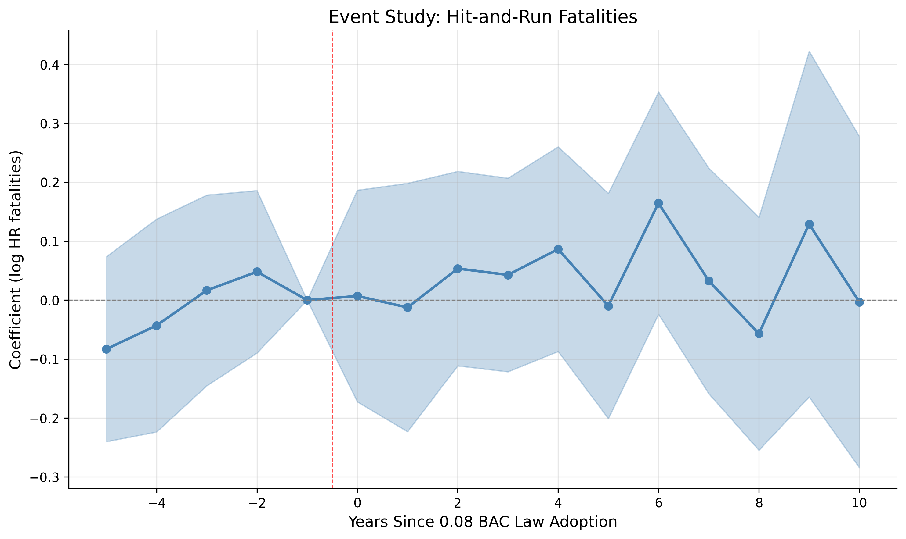
Event study coefficients with 95% confidence intervals. Reference period: t = -1 (normalized to zero).
Reading This Plot
- Each dot is a coefficient estimate—the effect at that time relative to treatment
- Vertical bars are 95% confidence intervals. If they cross zero, the effect is not statistically significant
- The red dashed line marks t=0 (when the 0.08 BAC law took effect)
- t = -1 is missing because it's the reference period (all other coefficients are relative to this point)
Interpreting the Results: What Does This Event Study Tell Us?
Let's walk through what this plot is actually telling us.
Step 1: Check Pre-Treatment Coefficients (Parallel Trends)
Question: Were treated and control states on similar trajectories before the law changed?
What to look for: Coefficients at t = -5, -4, -3, -2 should be:
- Close to zero (bouncing around the horizontal line)
- Statistically insignificant (confidence intervals crossing zero)
- Not trending upward or downward
In our plot: The pre-treatment coefficients are generally small and not significantly different from zero. There's no obvious upward or downward trend before treatment. This supports our parallel trends assumption—hit-and-run rates weren't already diverging before states adopted stricter BAC laws.
Step 2: Check for Anticipation Effects
Question: Did behavior change before the law officially took effect?
What to look for: Coefficients at t = -2, -1 that are large or significant would suggest people anticipated the policy (maybe it was announced in advance, or there was media coverage).
In our plot: The coefficients right before treatment (t = -2, -3) are close to zero. This suggests drivers didn't change their behavior in anticipation of the law—the effect only kicks in when the law actually takes effect.
Step 3: Examine the Post-Treatment Effect
Question: What happened to hit-and-run crashes after the 0.08 BAC law was adopted?
What to look for:
- Direction: Are coefficients positive (increase) or negative (decrease)?
- Magnitude: How large are the effects? (Remember: if Y is in logs, coefficients are roughly percent changes)
- Significance: Do confidence intervals exclude zero?
- Dynamics: Does the effect appear immediately? Grow over time? Fade out?
In our plot: Post-treatment coefficients are positive—hit-and-run crashes increased after states adopted stricter BAC laws. The effect appears to grow over time rather than appearing immediately, suggesting a gradual behavioral adjustment. By 5+ years after adoption, hit-and-run crashes are noticeably higher in treated states.
Putting It All Together: The Story
This event study tells a coherent story:
- Before the law: Treated and control states had similar hit-and-run trends (parallel trends ✓)
- No anticipation: Behavior didn't change before the law took effect (no anticipation ✓)
- After the law: Hit-and-run crashes increased in states that adopted 0.08 BAC limits
- The effect grew over time: Suggesting a gradual behavioral response, not a one-time shock
The interpretation: Stricter drunk driving penalties created an unintended consequence. When caught drunk driving became more costly, some drivers who caused crashes chose to flee the scene rather than face the harsher penalties. The policy reduced the expected punishment for drunk driving crashes—but only if you can escape before police arrive.
⚠️ Caution: What This Doesn't Tell Us
Event studies are powerful but not bulletproof. Flat pre-trends are necessary but not sufficient for causal identification. There could still be time-varying confounders that happen to coincide with treatment timing. The identifying assumption (parallel trends in the absence of treatment) is fundamentally untestable—we can only check whether it's plausible, not whether it's true.
9. What Did We Learn?
The Results
Consistent with French & Gumus (2024), we find that 0.08 BAC laws are associated with an increase in hit-and-run fatalities. The event study shows the effect grows over time, suggesting a persistent behavioral response where drunk drivers flee crash scenes to avoid stricter penalties.
The Bigger Picture: How Research Actually Works
If you followed this example from start to finish, you've seen that empirical research involves a lot of mundane decisions: Which datasets to use? What unit of analysis? How to handle missing values? These decisions matter, and making them well requires understanding your research design.
Here's a mental checklist for your own projects:
- Start with the triangle: You need a question, data, and identification. Make sure you have all three before writing code.
- Think about units: Your treatment varies at some level (state-year in our case). Your analysis should probably be at that level too.
- Aggregate and merge carefully: Most bugs happen here. Understand what each merge should do.
- Look at your data: Descriptive stats catch errors and build intuition.
- Test your assumptions: The event study isn't just for publication — it tells you whether your design is credible.
Common Mistakes
- m:m merges: Almost always a mistake. Check for duplicates.
- Zeros coded as missing: State-years with 0 crashes should be 0, not missing.
- Wrong unit of analysis: Make sure all data is at the same level before merging.
- Forgetting to cluster SEs: Always cluster at the treatment level (state).
Replication Package
Download the complete replication package in your preferred language. Each package follows the standard project organization format with build/ and analysis/ folders:
Each package includes: master script, build scripts, analysis scripts, raw data, cleaned datasets, and output figures. Run the master script to reproduce all results.
Found something unclear or have a suggestion? Email [email protected].